Genetic Programming based Face Recognition
Hani M. Ibrahem
Department of Mathematics & Computer Science, Faculty of Science, Menoufia University,
Egypt
Mohammed M. Nasef
Department of Mathematics & Computer Science, Faculty of Science, Menoufia University,
Egypt
Mahmoud Emam
Department of Mathematics & Computer Science, Faculty of Science, Menoufia University,
Egypt
ABSTRACT
Face recognition is a high-dimensional pattern recognition problem. It has rapidly evolved and has become very popular in recent years. In this paper, an efficient technique for face recognition based on genetic programming is proposed. Genetic programming is an evolutionary computation technique that automatically solves problems without having to tell the computer explicitly how to do it. Features extracting is one of the most important steps in this technique. The main goal of this paper is to answer the question "Who am I?" Further, the proposed technique is not affected by face recognition aspects such as lighting condition, varying facial expression, and varying pose. The results demonstrate that the proposed technique can obtain better performances than other existing face recognition techniques.
General Terms
Pattern Recognition (Face Recognition).
Keywords
Face recognition, genetic programming, and geometric feature based method.
1.
INTRODUCTION
Over the last decade, face recognition has become one of the most active applications of visual pattern recognition due to its potential value for law enforcement, surveillance, and human-computer interaction [1]. Face recognition is used to identify one or more persons from still images or a video image sequence of a scene by comparing input images with faces stored in a database [2]. A number of approaches for face recognition and classification have been proposed in the literature. These can be classified as Principal Components Analysis (PCA) [3], Fisher’s Linear Discriminant (FLD) [4], Independent Components [5], Discriminative Common Vectors [6] and Laplacianfaces [7]. Face recognition is an unsolved problem under the conditions of pose, illumination, database size etc., still attracts significant research efforts [8].
Scientists would like to be able to give the computer a problem and ask the computer to build a program to solve it [9]. Genetic programming is an evolutionary computation technique that automatically solves problems without having to tell the computer explicitly how to do it. Furthermore, it can automatically create a general solution to a problem in the form of a parameterized topology [10]. It has never been used in face recognition domain although it has been used in classification and pattern recognition problems [11].
In this paper, an efficient and accurate technique based on genetic programming for face recognition is proposed. It is
robust in intrinsic conditions such as pose, illumination, facial expression, etc. The experimental results, on ORL (Olivetti Research Laboratory) database of faces [12], demonstrate that the proposed technique is effective for face recognition. The rest of the paper is organized as follows: A brief review of related work to face recognition given in Section 2. An introduction to genetic programming is provided in Section 3. Proposed technique with the experimental results is discussed in Section 4. Finally, the conclusions are summed up in Section 5.
2.
A REVIEW OF RELATED WORK
The Most successful approaches to frontal face recognition are eigenface [13], fisherface [4], neural network [14], dynamic link architecture [15], hidden Markov model [16]. Since, eigenface is one of the most applicant approaches to face recognition [2]. It is also known as karhunen-loeve expansion, eigenpicture, eigenvector, or principal component analysis (PCA). Any face image could be approximately reconstructed by a small collection of weights for each face and a standard face image (eigenface). The weights of each face are obtained by projecting the face image onto the eigenface. In mathematical terms, eigenfaces are the principal components of the distribution of faces, or the eigenvectors of the covariance matrix of the set of face images. The eigenvectors are ordered to represent different amounts of the variation, respectively, among the faces. Each face can be represented exactly by a linear combination of the eigenfaces. It can also be approximated using only the "best" eigenvectors with the largest eigenvalues. The best M eigenfaces construct an M dimensional space, i.e., the "face space"[2]. Eigenface appears as a fast, simple, and a practical method. But, in general, it does not provide invariance over changes in scale and lighting conditions.
Sarawat Anam et al. [17] proposed a computational model for face recognition using the concept of genetic algorithm and Back-propagation Neural Network. This method consists of, three steps, pre-processing step that includes face acquisition, filtering, clipping, and edge detection. Second step is features extraction that extracts the features of the face images. Third step is recognition; in this step the extracted features have been fed into the genetic algorithm and Back-propagation Neural Network. Sarawat Anam et al. reported that the maximum efficiency is 82.61% for face recognition system using genetic algorithm but 91.30% using Back-propagation Neural Network.
used to extract features from the images. Secondly, genetic programming is used to classify image groups and a leveraging method is used to improve the results. Both of eigenface method in [18] and recognition method in [11] was tested on ORL database of faces. So, these two methods are used in the comparison with the proposed method.
3.
GENETIC PROGRAMMING
Genetic programming is a collection of methods for the automatic generation of computer programs that solve carefully specified problems. It is an evolutionary computation technique that automatically solves problems without having to tell the computer explicitly how to do it [10]. Technically, it is a special evolutionary algorithm where the individuals in the population are computer programs. So, generation by generation genetic programming iteratively transforms populations of programs into other populations of programs [19]. Genetic programming constructs new programs by applying genetic operations which are specialized to act on computer program.
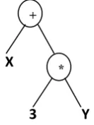
[image:2.595.135.202.432.521.2]Genetic programming operates with very general, hierarchical computer programs [10]. These programs have just one syntactic form called Symbolic expression (S-expression). It is equivalent to the parse tree for the computer program. Genetic programming trees and their corresponding expression can equivalently be represented in prefix notation [20]. Figure 1 shows the tree representation of the program x+3*y. The variables and constants (leaves of the tree) are called terminals, while the arithmetic operations (internal nodes) are called functions. Both of functions and terminals together form the primitive set of a genetic programming system.
Figure 1: A simple tree structure of genetic programming
When applying genetic programming to solve a problem, there are five major preparatory steps need to be specified [19, 21]. These steps are summarized as follows:-
1. Terminal set that includes the external inputs of a program, constants, and the zero-argument functions.
2. Function set that includes the statements, operators, and functions available to the genetic programming system (arithmetic functions, mathematical functions, Boolean functions, conditional functions, and iteration functions).
3. Fitness function is used to summarize how close a given design solution is to achieving the set aims. It is a numeric value assigned to each member of a population to provide a measure of a solution to the problem. The goal of having a fitness evaluation is to give a feedback to the learning algorithm regarding which individuals should have a higher probability of being allowed to reproduce and which
individuals should have a higher probability of being removed from the population. Fitness can be measured in many ways depends on the problem's type such as the amount of error between its output and the desired output, the amount of time required to bring a system to a desired target state, and the accuracy of the program in recognizing patterns or classifying objects.
4. Control parameters such as the population size, the probabilities of the genetic operations, and the maximum size for programs
5. Termination criterion is a predefined number which include a maximum number of generations to be run or it is an error tolerance on the fitness.
The first step to run a genetic programming is to initialize the population. Trees are the most common representation in genetic programming so; the syntactically valid trees must be constructed. The main parameter for the initialization method is the maximum tree depth. There are different methods for generating the random initial population [22]. The Grow and Full methods are considered to be the two simplest methods [9, 19]. In both grow and full methods, the initial individuals are generated so that they do not exceed a specified maximum depth in the tree. Grow method can be summarized as follows [9]:-
1. Starting from the root of the tree, every node is randomly chosen as either a function or terminal.
2. If the node is a terminal, a random terminal is chosen.
3. If the node is a function, a random function is chosen, and that node is given a number of children equal to the arity (number of inputs) of the function. For every one of the function’s children the algorithm starts again, unless the child is at depth m, in which case the child is made a randomly selected terminal.
Also, full method can be summarized as follows [9]:-
1. Every node, starting from the root, with a depth less than d, is made a randomly selected function. If the node has a depth equal to d, the node is made a randomly selected terminal.
2. All functions have a number (equal to the artily of the function) of child nodes appended, and the algorithm starts again. Thus, only if d is specified as one, could this method produce a one-node tree.
The main genetic operations involved in genetic programming are the following:
1. Crossover: the creation of one or two offspring programs by recombining randomly chosen parts from two selected programs.
2. Mutation: the creation of one new offspring program by randomly altering a randomly chosen part of one selected program.
3. Selection: the first step of each generation is the selection of parents from the current population. This method is based on the fitness function which is the metric for genetic programming evaluation. After the quality of an individual has been
+
*
Y
3
determined, we have to decide whether to apply genetic operators to that individual and whether to keep it in the population or allow it to be replaced. There are many methods for how to select the best parents, such as roulette wheel selection [23], rank selection [23, 24], and tournament selection [23, 25].
Finally, the general implementation of genetic programming algorithm can be summarized as the following algorithm [19].
Algorithm 1:
4.
PROPOSED METHOD
The most important goal in many areas such as artificial intelligence is to have computers automatically solve problems. So, genetic programming that defined as an evolutionary computation technique that automatically solves problems, is achieving this goal. A technique for face recognition based on genetic programming is proposed in this section. The ORL database of faces [12] is used to evaluate the performance of the proposed technique. It consists of 400 images with 10 different images for each of the 40 distinct individuals. The images vary across pose, size, time, and facial expression. The images were taken against a dark homogeneous background with the subjects in upright, frontal position with a tolerance for some tilting and rotation of up to about 20◦. Scale varied up to about 10%. The spatial and gray-level resolutions of the images are 92×112 and 256, respectively.
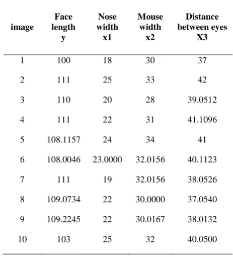
Extracting features from face images is one of the most important steps in this technique that can be categorized as a geometric feature based method. The significant facial features are detected and the distances among them as well as other geometric characteristics are combined in a feature vector for face representation. This vector is determined by four variables (y, x1, x2, x3) where,
y: is the face length.
x1: is the nose width.
x2: is the mouse width.
x3: is the distance between the eyes.
The proposed technique consists of two parts. Firstly, the feature vector of the face image is extracted then; genetic programming is applied on this vector to extract a mathematical formula for face representation. Secondly, the features are extracted from the input image and combined in a feature vector as previously. Then, this vector has been fed into the mathematical formula of all the stored faces in the
[image:3.595.401.455.110.170.2]database to find a match. The feature vector for the face image in Figure 2 is (108.0046, 23.0000, 32.0156, and 40.1123).
Figure 2: A sample of face image
The main goal is to use the feature vector to extract a mathematical formula using genetic programming. The formula appears as the function y = f(x1, x2, x3) that solves in y. After extracting the formula, the best match to the input face image is determined by comparing it with all stored faces in the database. Consider a number of stored face images with their mathematical formula. Consequently, the feature vector of the input image is fed into the mathematical formula of these stored images. If the y value of the input image is equal or nearest to the y value of a stored image, then the input image is matched this stored image.
[image:3.595.321.538.358.418.2]In the first part, the facial features of the face images are extracted and the distances among them are combined in a feature vector for face representation. Table 1 shows the feature vectors of the person in Figure 3.
Figure 3: An individual in the ORL database
Table 1. The feature vectors for the person in Figure 3
image
Face length y
Nose width x1
Mouse width
x2
Distance between eyes
X3
1 100 18 30 37
2 111 25 33 42
3 110 20 28 39.0512
4 111 22 31 41.1096
5 108.1157 24 34 41
6 108.0046 23.0000 32.0156 40.1123
7 111 19 32.0156 38.0526
8 109.0734 22 30.0000 37.0540
9 109.2245 22 30.0167 38.0132
10 103 25 32 40.0500
Then, genetic programming is applied on the data that obtained in Table 1 to extract the mathematical formula, for the individual in Figure 3, based on the number of the training images. Before apply this data to genetic programming the terminal set for feature vector (y, x1, x2, x3, and random 1: Randomly create an initial population of programs from
the available primitives. 2: Repeat
3: Execute each program and evaluate its fitness.
4: Select one or two program(s) from the population with a probability based on fitness to participate in genetic operations.
5: Create new individual program(s) by applying genetic operations with specified probabilities.
6: Until: an acceptable solution is found or reaching a maximum number of generations.
[image:3.595.311.543.447.703.2]integer numbers) and the function set for feature vector (+, -, *, and /) are defined. The main initiative parameters to create the program that defines the formula for the feature vectors are defined in Table 2. Figure 4 shows a part of the mathematical formula in S-expression for the feature vectors shown in Table 1 with 6 train images. The best-of-run individual program was found on generation 474 and had a standardized fitness measure of 3.015807E-8 with 6 hits (S-
expression).
[image:4.595.324.528.109.197.2]Table 2. Parameters used in the proposed technique for genetic programming run
Figure 4: A part of the mathematical formula in S-expression for the feature vectors shown in Table 1
with 6 train images.
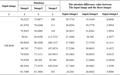
In the second part, a comparison between the input image and all stored images to find the best match is achieved. Consider
a three face images, as shown in Figure 5, stored in the database and their feature vectors are shown in Table 3.
Figure 5: Three different face images
Then, genetic programming is applied on the data in Table 3 depending on the number of the training images to extract the mathematical formula for each individual. Consider the input image as shown in Figure 2 the results of evaluating the feature vector of the input image with the mathematical formula of the stored images, in Figure 5, are illustrated in Table 4. The absolute difference of y value for the input image and each of the three images is used to determine the matching. From Table 4, Image3 is matched the input image.
[image:4.595.53.291.216.707.2]B. Bozorgtabar and G. Rad [11] applied their proposed technique on ORL database. They reported a recognition rate of 63.5% at 5 training images and 67.5% at 9 training images by using genetic programming, whereas they reported a recognition rate of 91.5% at 5 training images and 92.5% at 9 training images by using a leveraged genetic programming. In addition, V. Akalin [19] applied Eigenface technique on ORL database and the recognition rate results are reported in Table 5. The recognition rate of the proposed technique with different numbers of training images is shown in Table 6.
Table 5. Recognition rate of Eigenface technique [12]
Table 6. The recognition rate of the proposed technique
No. of Training images
Recognition rate results of the proposed technique
5 76%
6 90%
7 91%
8 95%
9 98%
GP parameter Value / Type
Maximum number of
Generations: 500
Size of Population: 2000
Maximum depth of new
individuals: 6
Maximum depth of new
sub-trees for mutants: 4
Maximum depth of individuals
after crossover: 18
Fitness-proportionate
reproduction fraction: 0.1
Crossover at any point fraction: 0.1
Crossover at function points
fraction: 0.1
Number of fitness cases: 6
Selection method:
FITNESS-PROPORTIONATE- WITH-OVER-SELECTION
Generation method: FULL
No. of Training images Eigenface technique[12]
5 90%
6 92.50%
7 91.60%
8 91.20%
9 90%
. .
.
[image:4.595.54.289.226.691.2] [image:4.595.334.549.454.575.2] [image:4.595.339.547.612.735.2]Table 3. Feature vectors for image1, image2, and image3
Image1 Image2 Image3
y X1 X2 X3 y X1 X2 X3 y X1 X2 X3
75 19 30 33 88 21 33.0151 35.0143 100 18 30 37
75 19 32 33 88 21 34.0147 35 111 25 33 42
75 19 30 32 87.0517 21 34.0588 35.0571 110 20 28 39.051
75 19 30 32 88 21 31.0644 34.0147 111 22 31 41.109
76 19 31 32 87.2067 21 31.0644 34.2345 108.115 24 34 41
78 20 30 33.015 89 21 32.0156 34.0147 108.004 23 32.015 40.112
78 19 29 31 89.202 20.025 32.0156 33.1361 111 19 32.015 38.052
78.0577 20 30 33 89 22 32.0624 34 109.073 22 30 37.054
77 20 30.016 31.016 88 22 31.0161 34 109.224 22 30.016 38.013
77 20 31 33 88.8144 22.090
7 31.4006 34.2345 103 25 32 40.05
Table 4. The evaluation results of the input image with 6 train images
Input image
Database
The absolute difference value between The input image and the three images
Image1 Image2 Image3
y y y y Input-Image1 Input-Image2 Input-Image3
108.0046
78.2327 72.0877 100 29.7719 35.9169 8.0046
81.9752 78.6268 111 26.0294 29.3778 2.9954
79.5033 56.9685 110 28.5013 51.0361 1.9954
80.82 69.6396 112.3723 27.1846 38.365 4.3677
80.9042 80.4308 108.1157 27.1004 27.5738 0.1111
80.745 77.9231 107.8374 27.2596 30.0815 0.1672
78.8183 77.1111 103.9931 29.1863 30.8935 4.0115
79.9785 80.305 95.949 28.0261 27.6996 12.0556
80.2562 77.4379 109.2245 27.7484 30.5667 1.2199
81.7406 81.3404 103 26.264 26.6642 5.0046
5.
CONCLUSION
Face recognition is one of the most fundamental functions for many kinds of intelligent robots. The main goal for researchers is to implement recognition algorithms that are more efficient for face recognition. So, the aim of this paper is
[image:5.595.93.502.426.682.2]6 efficient and accurate for face recognition that is robust in
intrinsic conditions such as varying lighting condition, varying facial expression, varying pose, etc.
6.
REFERENCES
[1] Jie Zou, Qiang Ji, and George Nagy, “A Comparative Study of Local Matching Approach for Face Recognition,” IEEE Trans. on Image Processing, vol.16, no. 10, pp. 2617-2628,Oct. 2007.
[2] Yongsheng Gao, and Maylor K.H. Leung, “Face Recognition Using Line Edge Map,” IEEE Trans. on Pattern Analysis and Machine Intelligence, vol. 24, no. 6, Jun. 2002.
[3] H. Moon, P.J. Phillips, “Computational and performance aspects of PCA-based face recognition algorithms,” Perception, vol. 30, pp. 303-321, 2001.
[4] P. N. Belhumeur, J. P. Hespanha, D. J. Kriegman, “Eigenfaces vs. Fisherfaces: Recognition using class specific linear Projection,”IEEE Trans. on Pattern Analysis and Machine Intelligence, vol. 19, no. 7, 1997.
[5] M.S. Bartlett, J.R. Movellan, T.J. Sejnowski, “Face recognition by Independent Component Analysis,” IEEE Trans. on Neural Networks, vol. 13, no. 6, pp. 1450-1464, 2002.
[6] H. Cevikslp, “Discriminative Commom Vectors for face recognition,”IEEE Trans. on Pattern Analysis and Machine Intelligence, vol. 27, no. 1, Jan. 2005.
[7] X. He, S. Yan, Y. Hu, P. Niyogi, and H.J. Zhang, “Face recognition using Laplacianfaces,” IEEE Trans.on Pattern Analysis and Machine Intelligence, vol. 27, 2005.
[8] Neerja and Ekta Walia, “Face Recognition Using Improved Fast PCA Algorithm,” Congress on Image and Signal Processing, 2008.
[9] M. Walker, "Introduction to Genetic Programming",www.cs.montana.edu/~bwall/cs580/intro duction_to_gp.pdf , October 2001.
[10]J. R. Koza, “Genetic Programming on the Programming of Computers by Means of Natural Selection,” MIT Press, Cambridge, Massachusetts, 1992.
[11]Behzad Bozorgtabar, Gholam Ali Rezai Rad, “A Genetic Programming-PCA Hybrid Face Recognition Algorithm,” Journal of Signal and Information Processing, 2, 170-174, 2011.
[12]ORL (Olivetti Research Laboratory) Face Database,http://www.uk.research.att.com/facedatabase.ht ml
[13]M. Turk, and A. Pentland, “Eigenfaces for Recognition,” Journal of Cognitive Neuroscience 13 (1), pp. 71– 86, 1991.
[14]S. Lawrence, C. Lee Giles, A. C. Tsoi, and A. D. Back, “Face Recognition: A convolutional Neural Network Approach,” IEEE Trans. on Neural Networks, vol. 1 , no.8, pp. 98–113, 1997.
[15]M. Lades, J. Vorbruggen, J. Buhmann, J. Lange, C. V. D. Malburg, and R. Wurtz, “Distortion Invariant Object Recognition in The Dynamic Link Architecture,” IEEE Trans. Comput., vol. 42, no. 3, pp. 300–311, 1993.
[16]F. Samaria and S. Young, “HMM Based Architecture for Face Identification,” Image and Computer Vision, vol. 12, pp. 537-583, Oct. 1994.
[17]Sarawat Anam, Md. Shohidul Islam, M.A. Kashem, M.N. Islam, M.R. Islam, and M.S. Islam, “Face Recognition Using Genetic Algorithm and Back Propagation Neural Network,” Proc. of the International MultiConference of Engineers and Computer Scientists, vol I, IMECS 2009, March 18 - 20, Hong Kong, 2009.
[18]V. Akalin, “Face Recognition Using Eigenfaces and Neural Networks,” A thesis submitted to the graduate school of natural and applied sciences of the Middle East Technical University, December , 2003.
[19]William B. Langdon, Riccardo Poli, Nicholas F. McPhee, and John R. Koza, “Genetic Programming: An Introduction and Tutorial, with a Survey of Techniques and Applications,” Studies in Computational Intelligence (SCI) 115, pp927–1028, Springer-Verlag Berlin Heidelberg, 2008.
[20]Banzhaf, W., Nordin, P., Keller, R.E., Francone, F.D “Genetic Programming– An Introduction; On the Automatic Evolution of Computer Programs and its Applications,” Morgan Kaufmann, San Francisco, CA, USA, 1998.
[21]J. R. Koza, “Survey of genetic algorithms and genetic programming,” in WESCON Conf., Piscataway, NJ: IEEE, pp. 589–594, 1995.
[22]Langdon, W.B, “Size fair and homologous tree genetic programming crossovers,” GP&EM, 1(1/2), 95–119, 2000.
[23]S. N. Sivanandam, and S. N. Deepa, “Introduction to Genetic Algorithms,” Springer-Verlag Berlin Heidelberg, 2008.
[24]G. Renner, and A. Ekárt, “Genetic Algorithms in Computer Aided Design,” Computer Aided Design 35, pp. 709 – 726, 2003.