A New Technique for Finding Min-cut Tree
Ashwani Kumar
Dept. of Computer Science & Engineering
G. B. Pant Engg. College, Pauri, Uttarakhand, INDIA
Surinder Pal Singh
Dept. of CSE Maharishi Markandeshwar Engineering College, MMU,
Mullana, Haryana, INDIA
Nitin Arora
Dept. of CSE Women Institute of Technology, Dehradun,
Uttarakhand, INDIA
ABSTRACT
In this paper we propose a new approximation algorithm for calculating the min-cut tree of an undirected edge-weighted graph. Our algorithm runs in O(V2.logV + V2.d), where V is the number of vertices in the given graph and d is the degree of the graph. It is a significant improvement over time complexities of existing solutions. However, because of an assumption it does not produce correct result for all sorts of graphs but for the dense graphs success rate is more than 90%. Moreover in the unsuccessful cases, the deviation from actual result is very less (usually for less than 5% pairs) and for most of the pairs we obtain correct values of max-flow or min-cut.
Keywords
Undirected edge-weighted graph; min-cut tree; dense graphs; max-flow; min-cut
1.
INTRODUCTION
Graph connectivity is one of the classical subjects in graph theory, and has many practical applications, for example in chip and circuit design, reliability of communication networks, transportation planning and cluster analysis [1, 5]. Finding the minimum cut of an undirected edge-weighted graph is a fundamental algorithmic problem. Precisely it consists in finding a non-trivial partition of the graph’s vertex set V into two parts such that the cut weight, the sum of weights of the edges connecting the two parts, is minimum. Given an undirected edge-weighted graph G with vertex set V and edge set E, the problem is to build a tree such that
u, v
V the weight of the edge having minimum weight on the unique path connecting u and v in the tree represents the value of minimum cut of graph separating u and v. We call this tree Minimum-Cut Tree.In this paper we propose a new approximation algorithm for calculating the min-cut tree of an undirected edge-weighted graph. Our algorithm runs in O(V2.logV + V2.d), where V is the number of vertices in the given graph and d is the degree of the graph. It is a significant improvement over time complexities of existing solutions. However, because of an assumption it does not produce correct result for all sort of graphs but for the dense graphs success rate is more than 90%. Moreover in the unsuccessful cases, the deviation from actual result is very less (usually for less than 5% pairs) and for most of the pairs we obtain correct values of max-flow or min-cut.
2.
RELATED WORK
Gomory and Hu [3] proved that min-cut or max-flow between all pair of vertices in an undirected graph can be computed by doing n-1 max flow computations rather than the naive max-flow computations. All the algorithms for constructing
the Minimum-Cut Tree use n-1 minimum s-t cut (i.e. max flow) subroutines.
Gomory and Hu [3] solved the multi-terminal network flow problem in 1961 and proved that maxflow problems in an undirected network have at most n-1 distinct solutions. They represented these n-1 values using a tree, nodes of which were same as those of original network and edge-weights were those n-1 values. This tree is known in literature as Gomory-Hu tree or Min-cut tree. Gomory and Gomory-Hu [3] presented an algorithm for making min-cut tree of an undirected, edge-weighted graph time complexity of which was O(V*Complexity of solving a maxflow problem).
The fastest algorithm known so far for solving max flow problem between two specified vertices has the complexity O(V3). Therefore Min-Cut tree can be constructed in O(V4) using the algorithm proposed by Gomory and Hu [3]. In this paper we do not use max flow subroutine here; rather we present an approximation algorithm in which we first calculate an upper bound for each vertex and repeatedly relax it till it becomes minimum-cut value. This approximation algorithm has a significantly better running time than the fastest existing algorithm till now and gives surprisingly good results for dense graphs.
3.
INTRODUCTION
TO MIN CUT TREE
Given a graph G = (V, E) with vertex set V, edge set E and weight function w: E R. It can be shown that there are at most n-1 distinct min-cuts among the total pairs of nodes.
We represent these n-1 min-cuts by a (not necessarily unique) tree, called Min-Cut Tree, which always exists and has the following properties:
The nodes of the tree are the same as the nodes of the initial graph, (i.e. V). Each edge is assigned a value (not directly related to the weights of the initial graph).
For every pair s, t, we can find the min-cut value by following the (unique) path between s and t in the min-cut tree. Suppose that e is the edge with minimum value on that path. Then value (e) is also the min-cut value between s and t in the initial graph G.
To actually find the cut between s and t, we simply cut off the edge e of minimum value on the s-t path. The two connected subsets of nodes in the tree, also define the min-cut between s and t in the initial graph G.
3.1
Notation Used for Min Cut Tree
i.e. weight of the cut w(C) is the sum of the weights of the edges connecting the two parts.
s-t Cut: For two vertices s, t V s-t cut is a cut C such that s S and t S or vice versa i.e. cut C separates s and t.
Min s-t Cut: A Min s-t cut of graph G is a s-t cut having minimum weight among all s-t cuts of G.
Min Cut: A Min cut of graph G is a cut C having minimum weight among all cuts of G. More detailed, a minimum cut of an undirected graph G with edge weights is a set of edges with minimum sum of weights, such that its removal would cause the graph to become unconnected.
4.
EXISTING APPROACHES TO SOLVE
THE PROBLEM
4.1.
Gomory-Hu Algorithm
Gomory and Hu [3] showed that in a graph having n nodes, there can be only n-1 numerically different flows. So all flow can be deduced after only n-1 different flows have been computed. Consider a flow network with a minimum cut (A, A’) separating Ni and Nj, Ni A and Nj A’. Construct a
slightly different network, one in which all nodes in A’ are replaced by a single node P to which all the arcs of the cut are attached. In this condensed network consider the maximum flow between two ordinary nodes Ne and Nk. Gomory and Hu
proposed the following lemma:
Lemma: The flow between two ordinary nodes Ne and Nk in
the condensed network is numerically equal to the flow f(e, k) in the original network.
Gomory and Hu proposed the following method to compute the min-cut tree of an undirected, edge-weighted graph [3]: They take two nodes and do a maximal flow computation to find a minimum cut (A, A’). They represent this by two generalized nodes connected by an arc bearing the cut value. In one node are listed the nodes of A, in the other those of A’. They now repeat this process. Choose two nodes in a (or two in A’) and solve the flow problem in the condensed network in which A’ (or A) is a single node. The resulting cut has a value and is represented by a link connecting the two parts into which A is divided by the cut, say and . A’ is attached to if it is in the same part of the cut as , to if it is in the same part as .
The cutting up is then continued. At each stage we have certain generalized nodes (which may represent many nodes of the original network), and certain arcs connecting them. To proceed with the computation we select a generalized node and two original nodes in . Upon removing all arcs which connect to , the network of generalized nodes falls into a number of disconnected components. We condense each component except itself into a single node and solve the network flow problem consisting of these condensed nodes and the original nodes within , and using as source and sink. The minimal cut obtained by this flow calculation splits into two parts, . This is represented in the diagram by replacing by two generalized nodes connected by an arc bearing the cut value. All other arcs and generalized nodes in the
diagram are unchanged except those arcs which formerly connected to . Such an arc is now attached to if its component was on the same side of the cut as the nodes in , and attached to , if its component fell on the other side.
This process is repeated until the generalized nodes of the diagram consist of exactly one node each. This point is reached after exactly n-1 cuts, for the array is a tree at all times so when the process stops it is an n-node tree and so has n-1 branches each created by solving a flow problem in a network equal to or smaller in size than the original.
The algorithm proposed by Gomory and Hu has time complexity O (V*Time complexity of finding a min s-t cut).
4.2.
Finding Min s-t Cut
All the approaches to find min s-t cut till now use its close relationship to Maximum Flow Problem [1].
In the maximum flow problem we are given a flow network G = (V, E) which is a graph in which each edge (u, v) E has a non-negative capacity c(u, v) ≥ 0. If (u, v) E then it is assumed that c(u, v) = 0. We distinguish two vertices in a flow network: a source s and a sink t. In this problem we wish to compute the greatest rate at which material can be shipped from the source s to the sink t without violating any capacity constraints.
Let G = (V, E) be a flow network with a capacity function c. Let s be the source of the network, let t be the sink. A flow in G is a real valued function f : V x V R that satisfies the following three properties:
Capacity Constraint: For all u, v V, we require
f(u, v) ≤ c(u, v).
Skew Symmetry: For all u, v V, we require
f(u, v) = -f(v, u)
Flow Conservation: For all u V – {s, t}, we require
The quantity f(u, v), which can be positive, zero or negative is called the flow from vertex u to vertex v. The value of a flow f is defined as
4.2.1.
Ford-Fulkerson Method
The following Ford-Fulkerson method [4] is used for finding max flow between a pair of vertices s and t. This method is iterative. We start with f(u, v) = 0 for all u, v V, giving an initial flow of value zero. For each iteration we increase the flow by finding an “augmenting path”, which we can think of simply as a path from the source s to sink t along which we can send more flow, and then augmenting the flow along this path. We repeat this process until no augmenting path can be found.
Procedure: Ford-Fulkerson-Method(G, s, t)
Initialize flow to 0
While there exists an augmenting path p
do Augment flow f along p
return f
If we implement the computation of the augmenting path p with a breadth first search i.e. if the augmenting path is a shortest path from s to t in the residual network, where each edge has unit distance (weight), we call the Ford-Fulkerson method [4] so implemented the Edmonds-Karp Algorithm. Running time of Edmonds-Karp Algorithm is O(VE2). The asymptotically fastest maximum-flow algorithms are based on push-relabel method and have the running time of O(V3).
4.2.2.
Max-Flow-Min-Cut Theorem
The Max-Flow-Min-Cut theorem by Ford and Fulkerson shows the duality of the maximum flow and minimum s-t cut. This theorem states that the value of maximum flow in a flow network G with source s and sink t is equal to the value of min s-t cut of G.
So using the algorithm proposed by Gomory and Hu Min-Cut tree can be constructed in O(V4).
4.3.
Finding Overall Minimum Cut
M. Stoer and F. Wagner [1] have given a simple and compact algorithm for finding the minimum cut of a graph. The algorithm is remarkably simple and has the fastest running time so far. The algorithm uses the following very interesting theorem:
Theorem: Let s and t be two vertices of a graph G. Let G/{s, t} be the graph obtained by merging s and t. Then a minimum cut of G can be obtained by taking the smaller of a minimum s-t cut of G and a minimum cut of G/{s, t}.
So a procedure finding an arbitrary min s-t cut can be used to construct a recursive algorithm to find a min cut of a graph. To find an arbitrary min s-t cut this algorithm uses maximum adjacency search or maximum cardinality search.
Procedure: Min-Cut Phase (G, w, a)
A←{a} While(A≠V)
Add to A the most tightly connected vertex Store the cut-of-the-phase and shrink G by merging the two vertices added last.
A subset A of the graph vertices grows starting with an arbitrary single vertex until A is equal V. In each step, the vertex outside of A most tightly connected with A is added. Formally we add a vertex
zA such that w(A, z) = max{w(A, y)| yA},
where w(A, y) is the sum of the weights of all the edges between A and y. At the end of each such phase, the two vertices added last are merged, that is, the two vertices are replaced by a new vertex, and any edges from the two vertices to a remaining vertex are replaced by an edge weighted by the sum of the weights of the previous two edges. Edges joining the merged nodes are removed.
The cut of V that separates the vertex added last from the rest of the graph is called the cut-of-the-phase. The lightest of these cut-of-the-phases is the result of the algorithm, the desired minimum cut:
Procedure: Min Cut(G, w, a)
While(|V| > 1)
Min-Cut Phase(G, w, a)
if(the cut-of-the-phase is lighter than the current minimum cut)
then store the cut-of-the-phase as the current minimum cut
The starting vertex a stays the same throughout the whole algorithm. It can be selected arbitrarily in each phase instead. In order to prove the correctness of this algorithm they following lemma.
Lemma: Each cut-of-the-phase is a minimum s-t cut in the current graph, where s and t are the two vertices added last in the phase
Running time of the algorithm: The algorithm consists of |V| - 1 identical phases each of which requires O(|E| + |V| log |V|) time yielding an overall running time of O(|V||E| + log |V|).
5.
OUR APPROACH TO FIND MIN CUT
TREE
We present a new approximation algorithm [7] for constructing the minimum cut tree. We calculate an upper-bound value for each node in the graph[1]. We define the upper bound value of each node as the value of cut which separates this node from rest of the graph i.e.
Lemma:The value of minimum cut of a graph G separating Ni and Nj is less than or equal to minimum of the upperbound
Proof: Simple reasoning can be given to prove it. Let (A, A’) be the minimum cut of G separating Ni and Nj.
Upper-bound(Ni) and upper-bound(Nj) are the values of two cuts
which also separate Ni and Nj. Therefore,
w(A, A’) ≤ min(upperbound(Ni), upperbound(Nj))
where w(A, A’) =
Algorithm: We proceed by finding an edge uv such that upon merging the two nodes Nu and Nv we are able to reduce the
upperbound value, i.e.
upperbound(Nu) + upperbound(Nv) – 2*w(u,v) <
max(upperbound(Nu), upperbound(Nv))
We start from the node having the minimum upperbound value and check for all of the edges leaving it. If we are able to reduce the upperbound value by merging it with any of the nodes, we merge the nodes and repeat the same procedure. If we are not able to reduce the node’s upperbound value, we check for rest of the nodes in the increasing order of upperbound values. The reason behind considering the nodes in increasing order of upperbound values will be clear in the next lemma.
After all the nodes in the graph are merged and it has only one node left, we proceed to construct the min-cut tree by using the information from intermediate stages. We move from last to first stage and at each stage we see the two nodes that were merged during last stage and separate the node with smaller of the two upperbound values from the other by an arc bearing the value equal to the smaller of the two upperbound values. Since we separate the two merged nodes in the tree by an arc having the value equal to smaller of the two upperbound values, it is necessary to consider the nodes during merging process in the increasing order of upperbound values so that the node with less upperbound value will be merged first, if possible at all.
Lemma: If we consider the nodes to be merged in the increasing order of upperbound values and while examining the adjacency list of Ni we get Nj as the node which upon
merging with Ni will reduce the upperbound value of Ni, then
(1) Either upperbound(Nj) will also be reduced.
(2) Or upperbound(Nj) can’t be reduced.
Proof: We are considering the nodes in the increasing order of upperbound values, and so
Case 1: upperbound(Nj) ≥ upperbound(Ni)
Since merging Ni and Nj reduces the upperbound
value of Ni, therefore
upperbound(Ni) + upperbound(Nj) – 2*w(i, j) ≤
upperbound(Ni)
It is clear from above two equations:
upperbound(Ni) + upperbound(Nj) – 2*w(i, j) ≤
upperbound(Nj)
i.e. upperbound(Nj) is also reduced.
Case 2: upperbound(Nj) < upperbound(Ni)
Since we are considering the nodes in the increasing order of upperbound values, checking for Ni itself implies that Nj has
already been checked and it was not possible to reduce its
upperbound value at all. So in this case upperbound(Nj)
cannot be reduced.
If at any stage it is not possible to merge any node, then we merge that pair of nodes which results in minimum increment of the upperbound value.
Assumption: Our algorithm is based on the assumption that if we are merging two nodes Ni and Nj and if upperbound(Ni) <
upperbound(Nj) then it is not possible to merge Nj with any
other node which will result in a node having upperbound value which is less than upperbound(Ni). However, this
assumption is not true always.
During the course of our algorithm, if we merge a pair of nodes Ni and Nj such that:
(i) upperbound(Ni) < upperbound(Nj) and,
(ii) It was possible to merge Nj with some other node Nk such that
upperbound value of the resulting node (let it be val) would have been less than upperbound(Ni),
In this case, the resulting min-cut tree will not be correct and will give wrong min-cut values for some pair of nodes. More precisely, it would give the value of min Ni-Nj cut as
upperbound(Ni) but the correct value is val. We call such a
pair of nodes wrong pair to merge.
For sparse graphs, the probability of choosing the wrong pair of nodes to merge is high due to the less number of available pairs among which to choose i.e. due to less number of edges. For dense graph, the probability of choosing wrong pair of nodes is very less due to large number of available pairs among which to choose i.e. due to large number of edges. For dense graph this algorithm produces surprisingly good results. After running the procedure with more than 20000 randomly generated graphs we have figured out that for graphs having density >= 0.4, success rate of algorithm is more than 90%. Moreover in the unsuccessful cases, the deviation from actual result is very less (usually for less than 5% pairs) and for most of the pairs we obtain correct values of max-flow or min-cut.
Procedure: Min-Cut Tree(G)
Input: Undirected edge-weighted graph G Output: Min-Cut Tree
1. Calculate the upperbound values for each node. 2. while(number of vertices in the current graph > 1) 3. loop(Consider the vertices in the increasing order of upperbound value)
4. if(upperbound value can be reduced by merging a node with any adjacent node)
5. then merge those two adjacent nodes 6. break;
7. End if
8. End loop
9. if (it is not possible to merge any pair of nodes) 10. then merge the pair of nodes which results in minimum increment of the upperbound value.
11. End if
13. Construct Min-Cut Tree T by using the information from intermediate stages as described:
a. Move from last to first stage.
b. At each stage check the two nodes that were merged during last stage.
c. Separate the node with lower upperbound value from the other by an arc bearing the value equal to the lower upperbound value.
14. return T
Time Complexity: O(V2.logV + V2.d)
where V is the number of vertices in the given graph and d is the degree of the graph.
6.
RESULTS ANALYSIS
6.1
Random Graphs with Fixed Number of
Nodes
[image:5.595.60.532.208.397.2]We generated 7500 random graphs of different densities but having fixed number of nodes (=50). Edge-weights were also random and were in between 1-300. Results of running our algorithm with these graphs are summarised in following plots:
Fig 1: Plot of Success Rate Vs Density (Number of nodes were fixed to 50)
It is clear from figure 1 that for desity >= 0.4 success rate is about 100%. Figure 2 says that for the unsuccessful test cases deviation from the actual result is less than 3%. It means that
even in the case of failure we get correct valus of max-flows or min-cuts for most of the pair of nodes.
[image:5.595.63.533.484.670.2]
6.2.
Random Graphs with Random
Number of Nodes
We generated 7500 random graphs of different densities and number of nodes in them were also random (=5-55). Edges weights were also random and were in between 1-300.
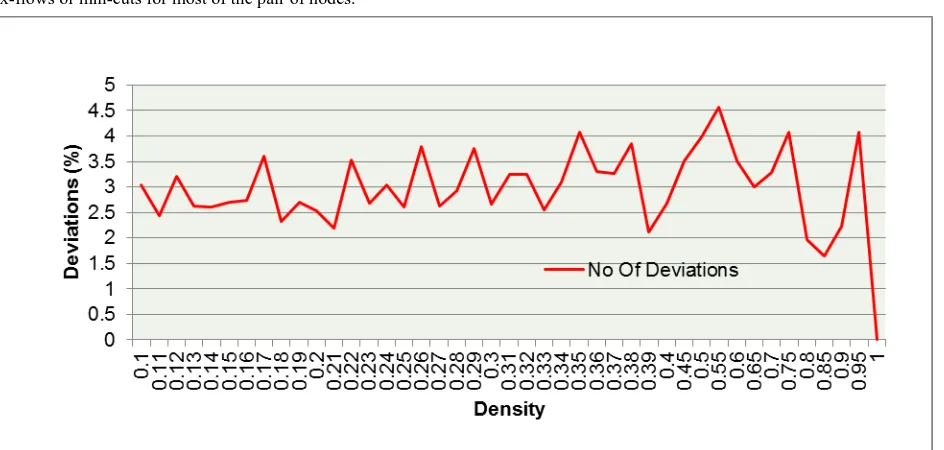
[image:6.595.53.529.143.327.2]Results of running our algorithm with these graphs are summarised in following plots:
Fig 3: Plot of Success Rate Vs Density (Number of nodes were random 5-55)
It is clear from figure 3 that for desity >= 0.4 success rate is more than 92%. Figure 4 says that for the unsuccessful test cases deviation from the actual result is less than 5%. It means that even in the case of failure we get correct valus of max-flows or min-cuts for most of the pair of nodes.
[image:6.595.65.537.430.655.2]7.
CONCLUSION
Approximation algorithm presented in this paper for calculating the min-cut tree of an undirected edge-weighted graph runs in O(V2.logV + V2.d), where V is the number of vertices in the given graph and d is the degree of the graph. This algorithm shows a significant improvement over time complexities of existing solutions. For the dense graphs success rate of our algorithm is more than 90% and because of an assumption it does not produce correct result for all sorts of graphs. Moreover in the unsuccessful cases, the deviation from actual result is very less (usually for less than 5% pairs) and for most of the pairs we obtain correct values of max-flow or min-cut.
8.
REFERENCES
[1] Arora N., Kaushik P. K. and Singh S. P., “A Survey on Methods for finding Min-Cut Tree”. International Journal of Computer Applications (IJCA), Volume 66, No. 23, March 2013, pp. 18-22.
[2] Stoer M. and Wagner F. “A Simple Min-Cut Algorithm”. Journal of the ACM (JACM), Volume 44, No. 4, July 1997, pp. 585-591.
[3] Brinkmeier M. 2007. “A Simple and Fast Min-Cut Algorithm”. Theory of Computing Systems, Volume 41, issue 2, pp. 369-380.
[4] Gomory R. E. and Hu T. C. December 1961. “Multi-Terminal Network Flows”. J. Soc. Indust. Appl. Math, volume 9, No. 4. [5] L. R. Ford and D. R. Fulkerson. Maximal Flow through a
network. Can. J. Math., 8:399-404, 1956.
[6] Hu T. C. 1974. “Optimum Communication Spanning Trees”. SIAM J. Computing, volume 3, issue 3.
[7] Flake G. W., Tarjan R. E. and Tsioutsiouliklis K. “Graph Clustering and Minimum Cut Trees”. Internet Mathematics, volume 1, issue 4, 385-408.