Evaluation of Tuning and Normalized Tuning time using
an Effective and Automated Framework pertained to
Benchmark Applications
J.Andrews
Research Scholar Sathyabama University
Chennai, India
T.Sasikala,
PhD. PrincipalSRR Engineering College Chennai, India
ABSTRACT
Tuning compiler optimization for a given application of particular computer architecture is not an easy task, because modern computer architecture reaches higher levels of compiler optimization. These modern compilers usually provide a larger number of optimization techniques. By applying all these techniques to a given application degrade the program performance as well as more time consuming. The performance of the program measured by time and space depends on the machine architecture, problem domain and the settings of the compiler. The brute-force method of trying all possible combinations would be infeasible, as it’s complexity O(2n ) even for “n” on-off optimizations. Even though many existing techniques are available to search the space of compiler options to find optimal settings, most of those approaches can be expensive and time consuming. In this paper, machine learning algorithm has been modified and used to reduce the complexity of selecting suitable compiler options for programs running on a specific hardware platform. This machine learning algorithm is compared with advanced combined elimination strategy to determine tuning time and normalized tuning time. The experiment is conducted on core i7 processor. These algorithms are tested with different mibench benchmark applications. It has been observed that performance achieved by a machine learning algorithm is better than advanced combined elimination strategy algorithm.
General Terms
Compiler Optimization, Machine learning
Keywords
Machine learning, Program features, Compiler optimization, Mibench
1.
INTRODUCTION
Modern architecture designer strives to bring satisfactory system level performance by applying minimal power across a wide range of applications. But many compilers fail to deliver its performance because of rate of change in hardware evolution. A compiler usually provides a larger number of optimization options, from which users has to pick up best set of available options for a given application. Those who do not have in depth understanding of the compiler options, and interactions among compiler options, then it is really difficult to pickup best set of options. Compilers usually provide three
2.
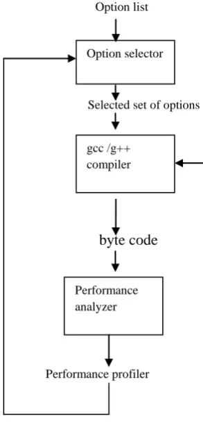
OPTIMIZATION SELECTION
STRATEGY
Option list
Selected set of options
byte code
[image:2.595.93.240.100.406.2]
Performance profiler
Fig 1: Optimization Selection .
3.
OPTIMIZATION SELECTION
ALGRITHMS
Given a set of “n” ON-OFF optimization options{F1,F2…Fn),find the best combination of flags that
minimizes application execution time and compilation time. In this paper a novel performance tuning algorithm advanced combined elimination algorithm is compared with a machine learning algorithm which picks up best set of options to improve tuning time and normalized tuning time.
3
.1 Advanced Combined Elimination Strategy
Let S be the set of available optimization options Let B represents selected compiler options set. i) Find TB ,by applying all flags are ON.
ii) Compile the program with TB configuration and measure
the program performance.
iii) Calculate Relative improvement percentage (RIP) for each and every optimization options. Relative improvement percentage is calculated based on finding the time required by applying particular flag ON and OFF with respect to TB.
iv) Store all the values in an array based on ascending order.i.e the most negative RIP is stored in first position of the array.
v) Remove the first two most negative RIP’s from an array instead of one. Now the value of TB is changed in this step.
vi) Remaining values in an array i.e i vary from 3 to n, Calculate RIP, and store the negative RIP’s in array.
v) If all values in an array represent positive values then set of flags in B represents best set.
Else
iv) Repeat steps ii until B contains only positive values. v) Stop
3.2 Machine Learning Algorithm
The Logistic Regression Model is a machine learning [3],[5] technique used to pick up set of options from a trained dataset. For a larger benchmark applications, finding the best set of compiler options will take more amount of time .To find a best set with less number of evaluations, we proposed a machine learning strategy. Collect set of program features for a given benchmark applications for a specific hardware during the training stage itself. For training we have collected more than 1000 set of combinations. These combinations compiled with gcc or g++ compiler and record the execution speed up. For collecting program features Intel Vtune performance profiler used. For collecting static program features Milepost GCC machine compiler used [2].The model is evaluated based on leave one out cross validation procedure.i.e if we have consider N=10(Where N is number of benchmark applications),i.e. the models are trained on N-1 benchmarks and tested on the Nth benchmark. The models were trained with 9000 points. The programs were compiled with 1000 sets of compiler setting and the performance is measured for a specific hardware platform. The various information such as compilation and execution time is stored on the repository. After training stage if a similar kind of program arrives by looking database one can who quickly searches best set of optimal settings.
4.
EXPERIMENTAL SETUP
In this paper we have considered GCC Version (4.3.2).GCC provides three levels of optimization techniques. Previous work considered only limited set of optimization techniques. In this paper more number of optimization techniques considered. Gcc compiler provides different levels of optimization techniques from –o0 to –o3.o3 is the highest level techniques. Level 1 consists of important techniques such as floop-optimize ,dead code elimination ,ftree-dce, dead store elimination, ftree-dse and scalar replacement of aggregates. Level 2 consists of important techniques such as global common sub expression elimination, gcse,peephole optimization, fpeephole2 and various basic block optimization techniques and scheduling optimization techniques .Level 3 consists of inline functions and unrolling. Although optimization level 3 (-O3) can produce faster code, the increase in the size of the binary image can have adverse effects on its speed.
4.1
Benchmark Applications
The Mibench benchmark [7], [10-11] suite programs were used to experiment the proposed algorithm. These benchmark suites are comparable with SPEC benchmark suite.
Option selector
gcc /g++ compiler
Bzip2: Bzip2 is a free and open source implementation of the Burrows–Wheeler algorithm. Bzip2 compresses most files more effectively than the older LZW (.Z) and Deflate (.zip and.gz) compression algorithms, but is considerably slower.Bzip2 compresses data in blocks of size between 100 and 900 kB and uses the Burrows-Wheeler transform to convert frequently-recurring character sequences into strings of identical letters. It then applies move-to-front transform and Huffman coding. bzip2 performance is asymmetric, as decompression is relatively fast. Bzip2 uses several layers of compression techniques stacked on top of each other, which occur in the following order during compression and the reverse order during decompression.
Consumer_jpeg_c: The JPEG standard allows "comment" (COM) blocks to occur within a JPEG file. Although the standard doesn't actually define what COM blocks are for, they are widely used to hold user-supplied text strings. This lets add annotations, titles, index terms, etc in JPEG files, and later retrieve them as text. COM blocks do not interfere with the image stored in the JPEG file. maximum size of a COM block is 64K.
consumer_tiff2bwTiff2bw converts an RGB or Palette color TIFF image to a grayscale image by combining percentages of the red, green, and blue channels. By default, output samples are created by taking 28% of the red channel, 59% of the green channel, and 11% of the blue channel. To alter these percentages, the -R, -G, and -B options may be used
qsort: The sort test sorts a large array of strings into ascending order using the well known quick sort algorithm. Sorting of information is important for systems so that priorities can be made, output can be better interpreted, data can be organized and the overall run-time of programs reduced. The small data set is a list of words; the large data set is a set of three-tuples representing points of data.
dijkstra:The Dijkstra benchmark constructs a large graph in an adjacency matrix representation and then calculates the shortest path between every pair of nodes using repeated applications of Dijkstra’s algorithm. Dijkstra’s algorithm is a well known solution to the shortest path problem and completes in O (n2) time.
patricia: A Patricia trie is a data structure used in place of full trees with very sparse leaf nodes. Branches with only a single leaf are collapsed upwards in the trie to reduce traversal time at the expense of code complexity. Often, Patricia tries are used to represent routing tables in network applications. The input data for this benchmark is a list of IP traffic from a highly active web server for a 2 hour period. The IP numbers are disguised.
Security blowfish: Blowfish is a keyed, symmetric block cipher, included in a large number of cipher suites and encryption products. Blowfish provides a good encryption rate in software and no effective cryptanalysis of it has been found
to date. However, the Advanced Encryption Standard now receives more attention. Blowfish is a general-purpose algorithm, intended as an alternative to the ageing DES and free of the problems and constraints associated with other algorithms.
susan :SUSAN is an acronym standing for Smallest Univalve Segment Assimilating Nucleus. For feature detection, SUSAN places a circular mask over the pixel to be tested (the nucleus). For corner detection, two further steps are used. Firstly, the centroid of the SUSAN is found. A proper corner will have the centroid far from the nucleus. The second step insists that all points on the line from the nucleus through the centroid out to the edge of the mask are in the SUSAN
.
4.2
Performance Metrics
Relative Improvement Percentage (RIP), RIP (Fi), which is the relative difference of the execution times of the two versions with and without Fi.
100
)
1
(
)
1
(
)
0
(
)
(
Fi
T
Fi
T
Fi
T
Fi
RIP
(1) If Fi=1 then Fi is ON, else OFF
The baseline of this approach switches on all optimizations.
TB=T(Fi=1)=T(F1=1,F2=1,…Fn=1),Where TB represents
base time.
%
100
)
0
(
)
0
(
Fi
T
Fi
TB
TB
RIP
(2)
If RIP (Fi=0) <0, the optimization of Fi has a negative effect, so it is better to turn off the function.
Tuning time:
It is the time taken by each probe, to determine the effect of individual options in a set of candidate options.
Normalized tuning time:
It is the time taken for computing time needed to check the effects of individual options.
NTT=tuning time for entire probe/(number of re executions*total candidates).Architecture used for testing was Intel Corei7 -2630 QM CPU 2.2Ghz.With 8GB RAM, using ubuntu operating system. And the compiler was GCC 4.3.2
5. RESULTS AND DISCUSSION
Table 2: Tuning Time in Seconds
S.No Benchmark
applications Ace
Machine Learning Algorithm
1. Bzip2 5.02 5.02
2. Consumer_jpeg.c 6.64 6.4
3. Consumer_tiff2bw 6.67 6.52
4. Network_dijkstra
0.65
0.66
5. Network_Patricia 2.95 2.72
6. Qsort 5.18 5.16
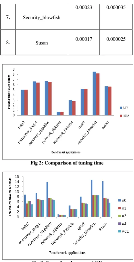
7. Security_blowfish 8.54 8.22
[image:4.595.65.397.68.735.2]8. Susan 5.67 5.6
Table 3: Normalized Tuning Time in Seconds
S.N o
Benchmark
applications Ace
Machine Learning Algorithm
1. Bzip2
0.00013 0.00002
2. Consumer_jpeg.c
0.00017 0.00003
3. Consumer_tiff2bw
0.00019 0.00003
4. Network_dijkstra
0.000025
0.00001
5. Network_Patricia
0.00008 0.00002
6. Qsort
0.00014 0.00003
7. Security_blowfish
0.00023 0.000035
8. Susan 0.00017 0.000025
Fig 2: Comparison of tuning time
[image:4.595.46.289.73.418.2]Fig 3: Execution time over ACE
Fig 5: Execution time over LRM
Fig 6: Comparison between different levels over ACE and LRM
In this section, we compare advanced combined elimination algorithm with a machine learning algorithm to find tuning time and normalized tuning time.Figure2 shows comparison of ACE and a machine learning algorithm. For most of the benchmark applications LRM gives least tuning time when compared to advanced combined elimination algorithm, because program features can be extracted and stored in a database..so if a similar program arrives with help of database one can quickly select best set of techniques. For some of the benchmark applications especially bzip2, dijkstra and qsort advanced combined elimination gives more or least tuning time when compared to LRM. Figure 3 shows comparison of execution time of different levels of GCC compiler optimization techniques with advanced combined elimination algorithm.GCC compiler consists of three different levels of optimization techniques. They are –o1,-o2 and highest level optimization techniques –o3.If by applying only the set of techniques from –o1 may reduce the compilation time but not so much of an performance on the execution time. So by considering set of techniques from –o2 improves execution time for most of the benchmark applications. By applying –o3 techniques for a given application may increase compilation and code size, but improves the program performance.
A good optimization algorithm should achieve both program performance and short tuning and short normalized tuning time. Figure 3 shows when compared to different levels of optimization techniques, ACE gives least execution
time for all the benchmark applications. Figure 4 shows comparison of normalized tuning time between ACE over LRM. Normalized tuning time is calculated by finding tuning time for each probe divided by number of re executions multiplied by total candidates. Table 3 shows normalized tuning time for every benchmark applications. Figure 5 shows execution time speed up between different levels of optimization techniques over LRM. Figure 6 shows combined execution time between ACE and LRM over different levels. From Figure 6 we can conclude that LRM achieves both program performance and short normalized tuning time for most of the benchmark applications.
6. CONCLUSION AND FUTURE SCOPE
In this paper, an alternative framework proposed for finding tuning time and normalized tuning time for Mibench benchmark applications. In this framework we have integrated Milepost GCC v2.1 and Intel Vtune performance analyzer for extracting program features upon training stage. These in formations are stored in a repository. So with the help of this information one can find best set of optimization techniques if a similar kind of program arrives. For this frame work we have implemented advanced combined elimination strategy. The results are compared with a machine learning algorithm. The results show that machine learning algorithm which improves the program performance, tuning time and normalized tuning time. In the future, we incorporate more compiler option selection algorithms to improve tuning time and normalized tuning time. In future we incorporate LLVM[12],ROSE[14] and path64[13] and other compilers in our framework. In future we include simulators in our framework to enable software and hardware optimization.7. REFERENCES
[1] GCC online documentation
http://gcc.gnu.org/onlinedocs/
[2] Grigori Fursin,Oliver Temam et al 2011.Milepost GCC:machine learning enabled self tuning compiler,,International journal on parallel programming,Springer,vol.39,pp.296-327.
[3] shih-Hao Hung, Chia-Heng Tu, Huang-Sen Lin,and Chi-Meng Chen2009,An Automatic Compiler Optimizations Selection Framework for Embedded Applications.In proceddings .of international .conference on Embedded Software and Systems,pp.381-387.
[4] Z.Pan and R.Eigenmann2006.Fast and effective orchestration of compiler optimizations for automatic performance tuning, In proceddings .of the international .symposium on code generation and optimization, pp.319-332.
[5] Agakov.F. Bonilla.E Cavzos and Williams 2006.Using machine learning to focus iterative optimization, In proceddings of the Intenational Symposium on code generation and optimization,pp.295-305.
[6] Chow.K and Wu.Y(2001),’Feed back directed selection and characterization of compiler optimization.
embedded benchmark suite,Workload characterization,2001.WWC-4.IEEE
International.workshop pp.3-14.
[8] William Von Hagen,2006.The definitive guide to
GCC’,Apress publications ,second
edition,ISBN:1590595858, pp.101-117.
[9] Brian J.Gough,2005.An introduction to GCC for gcc and g++ ‘,Revised edition,ISBN:0954161793,pp 45-53.
[10] www.networktheroy.co.uk
[11] www.sourceforge.net
[12] LLVM:the low level virtual machine compiler infrastructure.http://llvm.org
[13] Open64:an open source optimizing compiler.www.open64.net
[14] ROSE:www.rosecompiler.org.
![Cameron’s reality check on Europe. EPIN [Working] Paper No. 38, 15 April 2014](data:image/gif;base64,R0lGODlhAQABAIAAAP///wAAACH5BAEAAAAALAAAAAABAAEAAAICRAEAOw==)