http://dx.doi.org/10.4236/jcc.2015.311006
Semi-Supervised Dimensionality Reduction
of Hyperspectral Image Based on Sparse
Multi-Manifold Learning
Hong Huang1, Fulin Luo1, Zezhong Ma2, Hailiang Feng1
1Key Laboratory of Optoelectronic Technique and Systems, Ministry of Education, Chongqing University,
Chongqing, China
2Chongqing Institute of Surveying and Planning for Land, Chongqing, China
Received October 2015
Abstract
In this paper, we proposed a new semi-supervised multi-manifold learning method, called semi- supervised sparse multi-manifold embedding (S3MME), for dimensionality reduction of
hyper-spectral image data. S3MME exploits both the labeled and unlabeled data to adaptively find
neigh-bors of each sample from the same manifold by using an optimization program based on sparse representation, and naturally gives relative importance to the labeled ones through a graph-based methodology. Then it tries to extract discriminative features on each manifold such that the data points in the same manifold become closer. The effectiveness of the proposed multi-manifold learning algorithm is demonstrated and compared through experiments on a real hyperspectral images.
Keywords
Hyperspectral Image Classification; Dimensionality Reduction, Multiple Manifolds Structure, Sparse Representation, Semi-Supervised Learning
1. Introduction
Hyperspectral image (HSI) contains dozens or even hundreds of contiguous spectral bands, which has been widely used in land cover investigation [1]. However, the high dimensional characteristic of HSI will cause the curse of dimensionality [2]. Consequently, dimensionality reduction (DR) plays a critical role in HSI analysis, especially for the classification task when the number of available labeled training samples is limited.
In recent years, sparse representation (SR) has been successfully applied in HSI dimensionality reduction. SR aims at the sparse reconstructive weight which is associated with sample size. The representative methods in-clude sparse preserving projection (SPP) [3], discriminative learning by sparse representation (DLSP) [4] and discriminant sparse neighborhood preserving embedding (DSNPE) [5].
called sparse manifold clustering and embedding (SMCE) for simultaneous clustering and DR of data lying in multiple non-linear manifolds. While SMCE is also suffered from the out-of-sample problem, and they do not use the class information provided by training samples, which restricts their discriminating capability. Lu et al. [7] introduced a discriminative multi-manifold analysis method by learning discriminative features from image patches, which can perform well when label information is sufficient.
In the real world, the labeled samples are often very difficult and expensive to obtain. The supervised methods cannot work well when lack of training examples, in contrast, unlabeled examples can be easily obtained [8]. In such situations, it can be beneficial to incorporate the information which is contained in unlabeled samples into a learning problem, i.e., semi-supervised learning should be applied instead of supervised learning. At the same time, most of multi-manifold learning methods that have been applied to the processing of HSI rely either on supervised or unsupervised models, and only a few are focused on the semi-supervised setting.
To overcome the above drawbacks, we propose a new DR algorithm named semi-supervised sparse multi- manifold embedding (S3MME) in this paper. S3MME utilizes the merits of both sparsity property and multi- manifold learning to better characterize the discriminant property of the data. It exploits both the labeled and unlabeled pixels to adaptively find the local neighborhood of each data point by using an optimization program based on SR, and the selected neighbors are from the same manifold other than other manifolds. The weights associated to the chosen neighbors are automatically obtained simultaneously. It also exploits the wealth of la-beled samples in HSI data, and naturally gives relative importance to the lala-beled ones following a semi-super- vised approach. Then, an objective function pushes the homogeneous samples closer to each other is proposed, and the classification performance is further improved.
2. Semi-Supervised Sparse Multi-Manifold Embedding
Suppose that a HSI data set [ ,1 2, , ],m
N i
X = x x … x x ∈ℜ sampled from different manifolds { } c1
N i i=
, the first n points are labeled and the rest N−n points are unlabeled. Let li∈ …{1, ,Nc} denote the class label of xi. The
goal of DR is to map (X∈ℜm)(Y∈ℜd) by = T
Y V X, where dm. For supervised methods, only la-beled points are used for DR. While lala-beled and unlala-beled samples are used for semi-supervised methods.
We assume that naturally occurring data have possibly much fewer degrees of freedom than what the ambient dimension would suggest. Thus, we consider the case where the data lies on or close to multiple low-dimensional manifolds reside in a high dimensional space. To model the manifold structure of data, a similarity graph should be constructed, where nodes represent the data points and edges represent the similarity between data points. Then, a key issue for the similarity graph is to decide which nodes should be connected and how.
To achieve optimal discriminant features, each point will be connected to the points from the same manifold with appropriate weights, while the data pairs from different manifolds are disconnected. At first, for labeled points, we select the data points which have the same class label. Then, we formulate an optimization algorithm as in SMCE to find the unlabeled neighbors from the same manifold. Based on SR techniques, it selects a few da-ta points that are close to xi and span a low-dimensional affine subspace passing near xi. For labeled points, the points with the same class label and the unlabeled neighbors from the same manifold are used for the similarity graph. For unlabeled points, we try to find the neighbors which may come from the same manifold.
The sparse solutions { } 1
N i i
c = can be obtained by SMCE [6], where both labeled and unlabeled points are used. This motivates that for each data point xi to solve the following weighted sparse optimization program
2
1 2
1 min
2 i i i i Q c X c
λ + (1)
where the ℓ1-norm promotes sparsity of the solution, the proximity inducing matrix Qi is a positive-definite di-agonal matrix, and Xi denotes the matrix of normalized vectors {xj− xi}as follows:
( 1) 1
1 2 2
[ i n i ] m N
i
i n i
x x x x
X
x x x x
× −
− −
… ∈ℜ
− −
(2)
( 1) ( 1) 2
2
([ j i ] ) N N
i j i
t i t i x x Q diag x x − × − ≠ ≠ − ∈ℜ −
∑
(3)
The SR of each data point can be used for the construction of graph. Since the non-zero elements of {ci} are expected to come from the same manifold as of xi. We first construct a sparse graph Gs (V, E, Ws) with vertex set V = {xi, x2, …, xN}, edge set E, and symmetric weight matrix Ws. Then, we put an edge between nodes i and j if xi and xj are from the same class, or xi or xj is unlabeled but cij is a non-zero element.
Once the graph Gs is constructed, the affinity weight , [ , 1, , , ] N s i ws i ws iN
W … ∈ℜ of xi can be defined as
2 2
2 2
2 2
, 2 2
exp( ) exp( ), 0, ( )= ( )
2 2
exp( ) exp( ), 0,
2 2
0,
i i
i i
ij ij
ij i j i j
c d
ij ij
s ij ij i j
c d
c d
if c x or x is labeled and x x
t t
c d
w if c x or x is unlabeled
t t otherwise β ⋅ − ⋅ − ≠ = − ⋅ − ≠ (4)
where β is a trade-off parameter to adjust the contribution of labeled and unlabeled data,
0, 1 i ij d ij c j t d t ≠
=
∑
and0, 1 i ij d ij c j t d t ≠
=
∑
, t is the number of non-zero elements in ci.The obtained sparse graph built in this way has ideally several connected components, where points in the same manifold are connected to each other and there is no connection between two points from different mani-folds. In other words, the weight matrix of this graph has the following form
,1 ,
[ ] ([ [1], [2], , [ ]])
s s s N s s s c
W w w =diag W W W N (5)
where Ws[ ] is the weight matrix of data in , which includes the weight of labeled and some unlabeled
data.
The objective of S3MME is embodied as that it minimizes the sum of distances between data pairs which are expected to come from the same manifold. Then, a reasonable criterion for choosing an optimal projection vec-tor with stronger intra-manifold compactness on manifold is formulated as
2
, ,
min T i T j s[ , ] min ( T ( s[ ]) s[ ]) T ) min ( T s[ ]) T ) ij
x − x w ij = tr X − X = tr X X
∑
V V V V D W V V L V (6)
where xi and xj are related to the points in the same manifold which are connected to each other.
[ ] s
D is a diagonal matrix with s[ , ] s[ , ] j
D ii =
∑
w ij , and Ls[ ] =Ds[ ] −Ws[ ] is the Laplacian matrix.To remove an arbitrary scaling factor in embedding space, we impose a constraint to vectors V on , and the objective function on can be recast as
min tr(V X LT s[ ] X VT ), s.t. VTXDs[ ] XTV =I (7)
Then we apply the Lagrange multipliers to Eq. 7, we can get
, ,
[ ] T [ ] T
s i=λiX s X i
X L X v D v (8)
where v,i is the generalized eigenvector of [ ]
T s
X L X and XDs[ ] XT.
Let the column vectors v,0,v,1,…,v,d−1 be the solutions of Eq. (8) ordered according to their
eigenva-lues λ0 ≤λ1≤ … ≤λ,d−1. Thus, the embedding is given as follows:
, , , [ ,0, ,1, , , 1]
T
i i= i = … d−
,
Thus, we can use different weight matrix { [ ]} c1
N s =
W of the i-th manifold as a similarity between points in the corresponding manifold, and obtain a low-dimensional embedding of the data points.
3. Experiments and Discussion
3.1. Experimental Design
The goal of the experiments is to investigate the effectiveness of the proposed algorithms for classification of PaviaU hyperspectral data set. In each experiment, the data set was divided into training and test sets, and we randomly split the training set into the labeled and unlabeled set. The number of labeled samples l is varied as {10, 20, 40, 80} per class, while the number of unlabeled samples u is chosen in {100, 500, 1000, 2000, 3000}. For supervised DR methods, only the labeled set is used for training, while semi-supervised DR methods can utilize both labeled and unlabeled data. Then, all testing samples are projected into embedding space.
After that, reconstruction err classifier is used for multiple manifold classification [9], and nearest neighbor-hood (1-NN) is employed for other methods classification in all experiments. The classifier was evaluated against the test set, and we use overall classification accuracies (OAs) and the kappa coefficients (κ) to eva-luate the classification results. We repeat the classification process 10 times in each condition.
We compare S3MME with several representative DR algorithms such as PCA, LDA, LPP, LFDA, SPP, DLSP, DSNPE, semi-supervised sub-manifold discriminant analysis (S3MPE) [10] and semi-supervised discriminant analysis (SDA) [11]. The parameter β is set as 40 with cross-validation in S3
MME. Note that ε for SPP, DLSP and DSNPE is generally fixed across various instances of the problem, and we empirically set it to 0.1 in our experiments. For manifold learning methods, the number of nearest neighbors k is set to be 7. For all methods, the dimension of embedding features is set as 30.
3.2. Classification of PaviaU Data Set
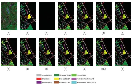
The PaviaU dataset was acquired by the reflective optics system imaging spectrometer (ROSIS) sensor during flight campaigns in 2003 over the Pavia University, northern Italy. It consists of 610 × 340 pixels and 115 spec-tral reflectance bands in the wavelength range 430-860 nm with a high spatial resolution of 1.3 m per pixel. Af-ter removing noisy and waAf-ter absorption bands, it reduced to 103 channels. Figure 1(a) shows a false color composite of the image, and Figure 1(b) shows the nine ground truth classes of interest.
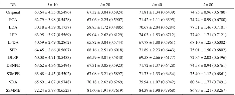
[image:4.595.88.540.539.722.2]In the first experiment, we evaluated the classification performance of S3MME. Table 1 reports the average classification performance achieved by different DR algorithms, where the OAs and the κ coefficients are dis-played for a varying number of labeled samples (10, 20, 40, 80 per class) and 3000 unlabeled samples. For illu-strative purposes, Figure 1 shows the classification maps obtained for different methods for the case of l = 40 per class and u = 3000 as in Table 1.
Table 1.OAs (in percent) and κ coefficients (in the brackets) with different numbers of labeled samples per class.
DR l = 10 l = 20 l = 40 l = 80
Original 63.64 ± 4.35 (0.5496) 67.32 ± 3.04 (0.5924) 71.81 ± 1.34 (0.6439) 74.75 ± 0.96 (0.6780)
PCA 62.79 ± 3.98 (0.5428) 67.06 ± 2.25 (0.5907) 71.42 ± 1.11 (0.6395) 74.74 ± 0.99 (0.6780)
LDA 30.18 ± 4.39 (0.1737) 58.85 ± 1.72 (0.4885) 70.67 ± 2.04 (0.6284) 77.51 ± 1.46 (0.7101)
LPP 63.95 ± 3.97 (0.5569) 69.04 ± 2.62 (0.6129) 74.03 ± 1.53 (0.6712) 77.49 ± 1.71 (0.7121)
LFDA 40.59 ± 2.69 (0.2862) 65.82 ± 3.04 (0.5744) 67.78 ± 1.80 (0.5961) 68.10 ± 1.25 (0.6002)
SPP 64.45 ± 2.66 (0.5607) 68.16 ± 2.51 (0.6018) 71.89 ± 2.23 (0.6443) 75.01 ± 1.50 (0.6802)
DLSP 60.08 ± 4.71 (0.5433) 66.59 ± 3.01 (0.5840) 69.58 ± 2.66 (0.6177) 72.35 ± 2.02 (0.6496)
DSNPE 63.62 ± 4.36 (0.5494) 67.31 ± 3.05 (0.5923) 71.72 ± 1.37 (0.6428) 74.58 ± 0.94 (0.6761)
S3MPE 63.68 ± 4.45 (0.5502) 67.08 ± 3.21 (0.5897) 71.73 ± 1.33 (0.6434) 75.40 ± 1.12 (0.6861)
SDA 65.69 ± 4.07 (0.5748) 70.18 ± 2.62 (0.6269) 75.94 ± 1.07 (0.6942) 80.54 ± 1.77 (0.7491)
Figure 1. Classification maps with different algorithms (l = 40, u = 3000). (a) False-color composition (bands 5, 40 and 15 for RGB); (b) Ground truth; (c) Labeled data; (d) Original (0.7411); (e) PCA (0.7407); (f) LDA (0.7527); (g) LPP (0.7746); (h) LFDA (0.6969); (i) SPP (0.7589); (j) DLSP (0.7244); (k) DSNPE (0.7410); (l) S3MPE (0.7453); (m) SDA (0.7862); (n) S3MME (0.8491). Note that OAs are given in parentheses.
As can be seen from Table 1, the classification performance improves for all methods as more data samples are used for training. The supervised methods, i.e. LDA and LFDA, degrade the performance of classification accuracy when the labeled sample size of training set is small, mainly due to the overfitting or overtraining. Our S3MME method produces better classification results than other methods in all situations, and the improvement is particularly significant when low number of labeled samples is used. The reason is that S3MME exploits the wealth of labeled and unlabeled samples to adaptively select neighbors from the same manifold and discovers the multi-manifold structure in HSI data, which respects both sparsity property and semi-supervised learning to better characterize the discriminant property of data.
By observing the classification results shown in Figure 1, the numerical results are confirmed by visual in-spection of the classification maps. The S3 MME method produces more homogenous areas and better classifi-cation maps than other methods, especially in Meadows, Trees, and Bare Soil.
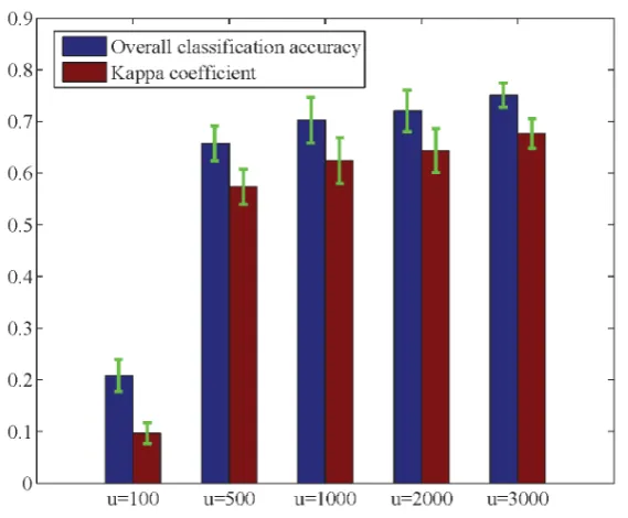
To investigate the influence of the numbers of unlabeled data on the performance of S3MME, we evaluate the classification accuracy using a small number of labeled samples (l = 10 per class) and different numbers of un-labeled samples (u = 100, 500, 1000, 2000, 3000), which are randomly selected for training. The classification results averaged over ten runs are shown in Figure 2.
An effective semi-supervised learning method can improve the performance when the number of the available unlabeled data increases. As expected, the OAs and κ coefficients of S3MME is significantly improved when the number of the available unlabeled data increases.
4. Experiments and Discussion
Figure 2. The classification results of S3MME using different numbers of unla-beled samples.
data points in the same manifold become closer. The S3MME method has been applied to a real hyperspectral image data set, and extensive experiments and comparisons have been conducted. Promising results have been obtained demonstrating the superiority of the proposed multi-manifold learning methods in hyperspectral image classification. The multi-manifold learning method proposed here are not utilize any spatial information in hyperspectral image. In our future work, we are going to consider the multi-manifold learning methods which make full use of both the spectral and spatial information provided by hyperspectral image.
Acknowledgements
This work is supported by National Science Foundation of China (41371338, 61101168), the Basic and Frontier Research Programs of Chongqing (cstc2013jcyjA40005), the Fundamental Research Funds for the Central Uni-versities of China (106112013CDJZR125501, 1061120131204), and Chongqing University Postgraduates’ In-novation Project (CYB15052). The authors would like to thank the anonymous reviewers for their constructive advice.
References
[1] Chen, Y., Nasrabadi, N. and Tran, T. (2013) Hyperspectral Image Classification via Kernel Sparse Representation.
IEEE Transactions on Geoscience Remote Sensing, 51, 217-231. http://dx.doi.org/10.1109/TGRS.2012.2201730
[2] Shao, Z. and Zhang, L. (2014) Sparse Dimensionality Reduction of Hyperspectral Image Based on Semi-Supervised Local Fisher Discriminant Analysis. International Journal of Applied Earth Observation and Geoinformation, 31, 122-129. http://dx.doi.org/10.1016/j.jag.2014.03.015
[3] Qiao, L., Chen, S. and Tan, X. (2010) Sparsity Preserving Projections with Applications to Face Recognition. Pattern Recognition, 43, 331-341. http://dx.doi.org/10.1016/j.patcog.2009.05.005
[4] Zang, F. and Zhang, J.S. (2011) Discriminative Learning by Sparse Representation for Classification. Neurocomputing,
74, 2176-2183. http://dx.doi.org/10.1016/j.neucom.2011.02.012
[5] Lu, G.F., Jin, Z. and Zou, J. (2012) Face Recognition Using Discriminant Sparsity Neighborhood Preserving Embed-ding. Knowledge-Based Systems, 31, 119-127. http://dx.doi.org/10.1016/j.knosys.2012.02.014
[6] Elhamifar, E. and Vidal, R. (2006) Sparse Manifold Clustering and Embedding. In: Advances in Neural Information Processing Systems, 609-616.
Training Sample per Person. IEEE International Conference on Computer Vision, 1943-1950.
http://dx.doi.org/10.1109/iccv.2011.6126464
[8] Shi, Q., Zhang, L.P. and Du, B. (2013) Semisupervised Discriminative Locally Enhanced Alignment for Hyperspetral Image Classification. IEEE Transactions on Geoscience Remote Sensing, 51, 4800-4815.
http://dx.doi.org/10.1109/TGRS.2012.2230445
[9] Wang, L.Z., Huang, H. and Feng, H.L. (2012) Multi-Linear Local and Global Preserving Embedding and Its Applica-tion in Hyperspectral Remote Sensing Image ClassificaApplica-tion. Journal of Computer-Aided Design & Computer Graphics,
24, 780-786.
[10] Song, Y.Q., Nie, F.P. and Zhang, C.S. (2008) Semi-Supervised Sub-Manifold Discriminant Analysis. Pattern Recogni-tion, 29, 1806-1813. http://dx.doi.org/10.1016/j.patrec.2008.05.024