Image Denoising by Addaptive Non Local Bilatetal Filter

Image Denoising by Addaptive Non-Local Bilatetal Filter

Dao Nam Anh

Electric Power University 235 Hoang Quoc Viet road

Hanoi, Vietnam

a. Image with Gaussian noise b. Result of Bilateral Filter c. Result of Non-Local Bilateral Filter Fig. 1. Denoise by bilateral filter and non-local bilateral filter.

ABSTRACT

In fields such as demosaicking, texture removal, dynamic range compression, and photo enhancement many imaging modalities operate with images corrupted by different noise models. Bilateral filter and non-local mean filter are often applied for deduction of noise. This paper presents a new adaptive bilateral filter model to reconstruct edges by choosing neighborhood with non-local mean concept. The method yields considerable gain reduction of noise and keep edges better than original method. Basing in visual inspection, the new method considered as effective even in case of mixed noise.

General Terms

Image processing

Keywords

Denoising, filtering, non-local mean, bilateral filter

1

INTRODUCTION

Image denoising is a major problem for noise reduction and image enhancement. As results, many methods had been proposed. Because noise and edges have common sign of high differential, preserve edges while remove different kind of noise requests more possible accuracy. Among the methods, bilateral filter and non-local mean are the success ones that remove noise and keep edges.

Bilateral filter proposed by Tomasi and Manduchi [1] is non-iterative, stable and simple method. It takes into account both space and intensity difference from the central pixel to suppress the noise and avoid edges diffusing.

Nonlocal means (NLM) denoising algorithms proposed by Buades et al in [2], which search neighborhood pixels in a relatively large search window, assign them weights by the similarity of intensity and average pixel intensities with the weights.

It is interesting to explore whether the neighborhood concept of NLM can be applied for bilateral filter and what influence it may have on performance of image denoising. In this paper, employability of NLM and bilateral filter for image denoising

with reserving edge is studied and a new adaptive bilateral filter is proposed with improved denoising quality.

A drawback of the original bilateral filter algorithm is the over smoothing of small sharp particles in the image. An example is illustrated in Figure 1: 1a displays image corrupted by Gaussian noise. The image filtered by the original bilateral filter is shown in figure 1b. The contrast between these small particles is smoothed. Figure 1c demonstrates result by the adaptive non-local bilateral filter that is presented in next sections.

2

OUTLINE OF PAPER

The rest of the paper is organized as follows. In the next section, related work and contributions are briefly reviewed. Major development of bilateral filter and non-local mean will be briefly presented. This is followed by a description of algorithm of adaptive bilateral filter for denoising in section 4. Section 5 provides some experimental results demonstrating the effectiveness of the proposed method. Discussion on the algorithm is tracked in section 6. Future work and some concluding remarks are given in section 7, 8.

3

CONTRIBUTIONS AND RELATED

WORK

Thanks to computational efficiency of bilateral filter, it attracts more and more research for its application [3], [4]. An example is Bilateral filtering framework for demosaicing with a means to denoise, sharpen, and demosaic the image simultaneously [5].

In [6] a bilateral filtering based mixture model with Markov Random Field (MRF) is introduced for image segmentation. The model incorporates spatial relationship among neighboring pixels into the Gaussian mixture model to perform a segmentation that is robust against noise.

a principal expression of the accuracy in terms of bandwidth and sampling. A subsequent post-processing and upsampling step using variations of cross-bilateral filtering is presented in [9]. The approach uses a combination of an initial disparity estimation and the line-wise hybrid recursive matcher. Porikli proposed methods that enable bilateral filtering in constant time ₍₁₎ without sampling [10]. First method takes advantage of the integral histograms to avoid the redundant operations. Second method uses linear filters of image powers without approximation. Third method expresses bilateral filters by Taylor series as linear filter decompositions. Averaging algorithms for realizing the bilateral filter in constant time are presented in [11], by using trigonometric range kernels, similar to polynomial kernels of Porikli [10]. Many researcher were attracted by non-local mean denoising algorithms [12],[13] like bilateral filters. Several alternative approaches were proposed to improve the method performance. Tanaka et al derived the common weighted average filter [14], with this both the bilateral filter and the NL-means filter can be interpreted as the patch-based posterior mean with the high-order MRF prior learned by the locally adaptive prior learning. Chatterjee et al presented a denoising framework through representation of image patches by learned basis functions [15]. Shimodaira proposed a patch-based bilateral filter [16] in which the intensity similarity is evaluated by comparing a whole patch around each pixel. Kervrann et al presented new Bayesian NL-means filter [17] where amount of smoothing is directly determined by the noise variance. In this filter, adaptive local dictionaries and a new statistical distance measure to compare patches are introduced.

Kim et al introduced a separable implementation of the nonlocal means filter and adopting a bilateral kernel for computing patch similarities [18]. Feng et al proposed non-local means framework based on neighborhoods’ gray value and the neighborhoods’ Gaussian curvature [19]. A non-local gradient-based energy for interpolating incomplete disparity maps is introduced by Lazcano et al [20]. It represents an extension of the bilateral filter adapted to reconstruct locally planar disparity maps.

In this paper bilateral filter is focused under concept of neighborhood of non-local filter. Next section presents a new adaptive bilateral filter with noise control improvement.

4

NON-LOCAL BILATERAL FILTER

Given _2_{, an image can be denoted as a M-dimension} function of space 

)) ( ),.. ( ( : ) ( ,

: u x u1 x u x

u M

N 

 

 , _2

x (1)

M i

ui:, 1,.., (2)

Let ube an observed image which includes pure signal

v

and additive noise n:

) ( ) ( )

(x v x nx

u   (3)

Denoising process is to obtain

v

from

u

.

4.1

Non-Local Mean

Buades et al defined a new intensity of pixel x as a weighted average of ufrom non-local pixelsyusing similarity weight functionw(x,y)depends on similarity of pixelsx and

y

[2]:

) ) .) ( .) ( ( exp( ) , ( ₂ 2 h y u x u G y x

w       (4)

.

is Euclide distance. Parameter h acts as a degree of filtering. The Gaussian filter G_ is a smoothing filter but at the cost of less distinct edges [21]:

      

 2₂

2 exp 2 1 ) (   

 x x

G (5)

From here non-local mean is defined as follows:





   ) ( ) ( ) , ( ) ( ) , ( ] [ x N y x N y x y x w y u y x w u NM (6)

whereN(x)is neighbours of x.

4.2

Bilateral Filter

Aurich and Weule [22] employed non-linear filters which combines the aspects of anisotropic diffusion and robust filtering basing on Gaussian filters:

   



       y x x W

A _{G y x G u y u x u y u x}

N x u u G r s )) ( ) ( ( ) ( ) ( || || ) ( ] [ .  

 (7)

with parameter _{[1,1.5]} to increase noise reduction, s



and

r



are filter scale of the spatial and intensity respectively.

x

N

is renormalization factor:







    ) ( )) ( ) ( ( || || x B y

x G x y u x v x

N

s 

 (8)

Tomasi and Manduchi introduced bilateral filter [1] with global constants

s



and

r



which smooths surfaces, just as the Gaussian Filter, while maintaining sharp edges in the image:











    S y x

x G x y G u x u y u y

W u BF

r

s || || ( ) ( ) ( )

1 ]

[ _{ } (9)

where |u(x)u(y)|is density difference in locations atx and

y





.

x

W is normalized weight at x:











    S y

x G x y G u x u y

W

r

s || ||  ( ) ( )

 (10)

For color image u(x):(u₁(x),u₂(x),u₃(x))











    S y y y x x

x G _s x y G_r

W u

BF[ ] 1 _ || || _ ||C C || C (11)

where ||CxCy|| is difference of color.

4.3

Non-Local Bilateral Filter for

Denoising Gray Image

With non-local concept from 4.2, bilateral filter (9) can has a new adaptive version as follows:











    ) (

*_{[ ]} 1 _{|| || ( ) ( ) ( )}

x B y x

x G x y G u x u y u y

W u BF r s    (12)











    ) ( ) ( ) ( || || x B y

x G x y G u x u y

where B(x)is set of neighbours of

x

that are similar to

x

. )

(x

B_ can be defined by similarity weight of Yaroslavsky et al [23], and Lee et al [24]:

) ) ( ) ( exp( ) , ( ₂ 2 h x u y u y x

w    (14)

or by (4) of Buades et al [2].

In this work, similarity function w(x,y) have simple L1 norm for discrete domain with a threshold



:

    _{ }  else false x u y u if true y x w , ) ( ) ( , ) , ( 1 _  (15) } ) , ( ), ( , { )

(x y y N x w x y true

B     (16)

The condition (15) is simple in comparison with (4) and (14) because the conditions of spatial neighborhood and intensity similarity are already presented in the first and the second Gaussian filter of the bilateral filter (12). The threshold



supports to refine neighbors selection with the most similar intensive value.

The search field yin (9) is replaced by yB_r(x)in (12) with non-local neighborhood by similarity weight

) , (x y

w_ . This is major introduction of non-local concept into a new adaptive bilateral filter. The concept is realized in the following algorithm.

ALGORITHM NLBF FOR DENOISING GRAY IMAGE

Given: Noise gray image u(x), initial _s,_r, parameter



. The denoising algorithm takes the following steps for each pixel x:

Step 1: Define its neighbors N(x)and then get similarity weight _w(x,y)for its neighbors by (15).

Step 2: Define similar neighbors B_(x)by (16). Step 3: Run bilateral filter

x

u

BF*[ ] by (12), (13) for x.

4.4

Denoising Color Image by Non Local

Bilateral Filer

Color image is presented by 3-D function u:

)) ( ), ( ), ( ( : ) ( ,

: 3 _{u x u}1 _{x u}2 _{x u}3 _x

u   , (17)

Where channel ui:,i1,2,3

Given initial global



_s,



_r, parameter



, similarity weight for each channel ui,i1,2,3is described:

    _{ }  else false x u y u if true y x w i i i , ) ( ) ( , ) , ( 1   (18)

non-local bilateral filter for each channel:











    ) ( *, ) ( ) ( ) ( || || 1 ] [ x B y i i i x x i

i s r

y u y u x u G y x G W u BF    (19)











    ) ( ) ( ) ( || || x B y i i i

x G x y G u x u y

W r s    (20)

where _Bi_{(x){y,yN}i_(x),wi_{(x,y)true}}



 (21)

ALGORITHM NLBF FOR DENOISING COLOR IMAGE

Given: Noise color image u(x), initial _s,_r, parameter



. The denoising algorithm takes the following steps:

For each channel ui,i1,2,3, for each pixel x

Step 1: Define its neighbors Ni(x)_{and then get similarity}

weight for its neighbors by (18). Step 2: Define similar neighbors Bi(x)

 by (21). Step 3: Run bilateral filter

x i _u

BF*[ ] _{by (19), (20) for x.}

5

EXPERIMENTS

5.1

Denoising Gray Image by NLBF

Using man image corrupted by different noise models to compare the proposed method with non-local mean [25],[26] and bilateral filter [1]. All the experiments are carried out on a 2.70 GHz PC with1.94 GB memory. The simulation software is Matlab R2011a.

The result is shown in fig. 4, there is input image with salt & pepper noise in fig 4a. Non-local mean gives result in fig. 4b, bilateral filter – fig. 4c, and non-local bilateral filter – fig. 4d. Fig. 4b keeps edges better than 4c, but it has more noise than 4c. Result 4d keeps edges well like 4b and deducts noise level of 4b.

Fig. 4e, 4f, 4g, 4h are for image corrupted by Gaussian noise. Fig. 4i, 4j, 4k, 4l – deals with speckle noise. The results of NLBF algorithm are better then other methods.

Improvement of denoising quality of new adaptive bilateral filter is shown in fig. 4d, 4g, 4l in comparison with original non-local filter (fig. 4b, 4f, 4j) and original bilateral filter (fig. 4c, 4g, 4k)

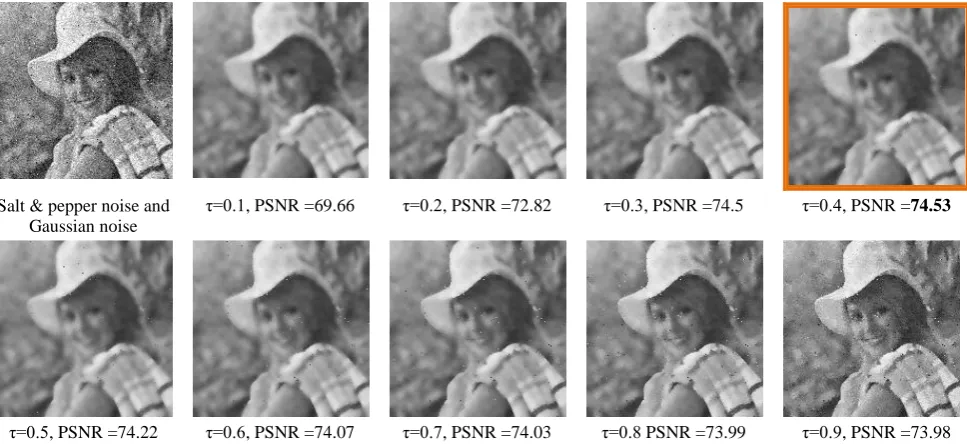
Figure 3 shows results of NLBF algorithm for different values of τ. Input image is corrupted by mixed noise: salt & pepper and Gaussian noise. The NLBF with parameter τ from .1 to .9 gives results in figure 3. Table 1 shows PSNR analysis for the each case. Peak Signal-to-Noise Ratio (PSNR) is the ratio between the reference signal and the distortion signal in an image. ) ( log 10 ) ( log

20 ₁₀ MAX ₁₀ MSE

PSNR  (22)

where MAX is the maximum possible pixel value of the image and MSE is the mean square error:



 

 

x u x v x

size

MSE _{( ( ) ( ))}2

) (

1 ₍₂₃₎

a. Input image with salt & pepper noise

b. Result of Non-local denoising filter for a.

c. Result of bilateral filter for a. d. Result of non-local bilateral filter τ =.1 for a.

e. Input image with Gaussian noise

f. Result of non-local filter for e.

g. Result of bilateral filter for e. h. Result of non-local bilateral filter by τ =.3 for e.

i. Input image with Speckle noise

j. Result of non-local filter for i.

[image:4.595.55.546.69.478.2]

k. Result of bilateral filter for i. l. Result of non-local bilateral filter by τ =.3 for i. Fig. 2. Effect of Non-local, Bilateral Filter and Non-local Bilateral Filter for gray “man” image

Salt & pepper noise and Gaussian noise

τ=0.1, PSNR =69.66 τ=0.2, PSNR =72.82 τ=0.3, PSNR =74.5 τ=0.4, PSNR =74.53

τ=0.5, PSNR =74.22 τ=0.6, PSNR =74.07 τ=0.7, PSNR =74.03 τ=0.8 PSNR =73.99 τ=0.9, PSNR =73.98

[image:4.595.56.540.510.732.2]

Image with noise

Bilateral filter

Non local

Mean Non local Bilateral Filter (NLBFilter)

[image:5.595.54.534.73.135.2]

(Noise Img) (BFilter) (NLM) τ=0.1 0.2 0.3 τ=0.4 0.5 0.6 0.7 0.8 0.9 PSNR 67.71 73.98 71.68 69.66 72.82 74.5 74.53 74.22 74.07 74.03 73.99 73.98

Table 1. Analysis of PSNR, for BF, NM, NLBF filters for gray “Girl” image with Salt & Pepper and Gaussian noise

A higher PSNR points out that the evaluated image is closer to the original image. The red line in the fig 4 displays effect of τ for the non-local bilateral filter.

The line of PSNR indicates that new filter with.4 gives output the most closest to the original image with

53 . 74



PSNR , higher than results of original non-local mean filter (71.68) and original bilateral filter (73.98). All three methods give PSNR higher than noise image (67.71).

1



 means selection of all neighbors, so the new filter products the same result like bilateral filter for the case.

Fig. 4. PSNR graph for Table 1

a. Input image with salt & pepper noise

b. Result of non-local filter for a

c. Result of bilateral filter for a. d. Result of non-local bilateral filter by τ =.3 for a.

e. Input image with Gaussian noise

f. Result of non-local filter for e.

g. Result of bilateral filter for e. h. Result of non-local bilateral filter by τ =.2 for e.

i. Input image with Speckle (Gamma) noise

j. Result of non-local filter for i

[image:5.595.296.543.80.294.2] [image:5.595.57.546.327.740.2]

Image/Filter Noise Img NLM BFilter NLBFilter τ =0.3 NLBFilter τ =0.4 NLBFilter τ =0.5

Girl 67.86 71.81 72.73 74.10 73.91 73.54

Mountain 67.99 70.22 68.47 71.08 70.33 69.60

[image:6.595.52.544.91.151.2]

Deer 67.83 72.26 74.62 75.81 75.77 75.33

Table 2.PSNR of non-local, bilateral filter and non-local bilateral filter for color BSDB images corrupted by mixed noise.

5.2

Denoising Color Image by NLBF

Color images of Berkeley Segmentation Dataset and Benchmark (BSDB) were selected to test with NLBF algorithm. Salt & pepper noise is appeared in input image (fig 5a). Results of non-local, bilateral filter and non-local bilateral filter are in fig. 5b, 5c, 5d. Figure 5e is an color image corrupted by Gaussian noise. Denoising by these methods give results in fig 5f, 5g, 5h. Similar test for speckle noise is demonstrated in figure 5i, 5j, 5k, 5l.

To check denoising quality, these color images was added salt & pepper noise and Gaussian noise and denoised by methods mentioned above. Table 2 resumes PSNRs of noise image and outputs of denoising methods. It shows that the best PSNR is from non local bilateral filter with τ =0.3. Graph in figure 6 illustrates the data of tables in columns. Example “mountain” has its PSNR columns in red. The best (highest) PSNR=71.08 is given by non local bilateral filter with τ =0.3

Fig. 6. Graph of PSNR of non-local, bilateral filter and non-local bilateral filter for color BSDB images corrupted

by mixed noise.

6

DISCUSSION

The algorithm NLBF needs three fixed parameters:

r s





, and



. Their values affect on performance of the algorithm. Parameters

r s





, regulate local Gaussian distribution of TV filter. Parameter



is used in step 2 of the algorithm to separate noise of edge. Wrong value of could lead to over-noise or over-edges. With experiments like examples in fig 3,



should be .3 or .4.

The bilateral filter (9) has computational complexity of

) (_nk2

O with size of imagenand size of search frame k. 2

k is result of double use of Gaussian function

G

_.

Computational complexity of non-local filter is O(n.2k), where the firstkis result of similarity function w(4) and the second kis get from neighbour distance calculation. For the

non-local bilateral filter (12), the complexity is ))

2 ( *

( 2

k k n

O  or simply_O(_nk2) _{as it combines}

neighbourhood condition with two Gaussian function

G

_.

7

FUTURE WORK

There are a few models of pure noise and mixed noise. Finding general method for denoising is an challenge. The algorithm NLBF was tested with three common noise models. It may need to check possibility of noise removing of the algorithm for other noise models.

8

CONCLUSION

This paper presents an attempt to improve bilateral filter for avoiding over smoothing of small sharp particles. Inspired by the neighborhood selection of non-local mean filter, a new adaptive bilateral filter is proposed. The new method is evaluated with original methods with BSDB color images. Experimental results confirm the improvement of the new adaptive non-local bilateral filter for denoising images. Basing in visual inspection, the new method considered as effective even in case of mixed salt & pepper and Gaussian noise. The nonlocal propagation capability of bilateral filter encourages future research for different applications.

9

ACKNOWLEDGMENT

Author thank Signal and Image Processing Institute, University of Southern California for USC-SIPI image database, two images from this were used in figure 2 and 3. We wish to thank Berkeley Computer Vision group for the BSDB, its images were used in figure 5 in this article. Special thank Douglas R. Lanman for his functions that implement 2-D bilateral filtering [25] with which codes for this article started.

Author would also like to thank the internal reviewers at EPU and the anonymous referees for their careful review and constructive comments.

10

REFERENCES

[1] C. Tomasi and R. Manduchi. Bilateral filtering for gray and color images. In Proc. of the Sixth International Conference on Computer Vision, Bombay, India, January 1998.

[2] Antoni Buades, Bartomeu Coll, Jean-Michel Morel, Image and movie denoising by nonlocal means, Image Processing On Line, 1 (2011).

[3] B. Weiss, Fast median and bilateral filtering, ACM Trans. on Graphics, vol. 25, no.3, pp. 519-526, 2006. [4] M. Elad, On the origin of the bilateral filter and the ways

to improve it, IEEE Trans. Image Process., vol. 11, pp. 141-1151, 2002.

[image:6.595.54.282.359.530.2]

segmentation, 19th IEEE International Conference on Image Processing (ICIP), 2012.

[7] Nagatsu Y, Katsura S, Macro–Micro Bilateral Control Using Kalman Filter Based State Observer for Noise Reduction and Decoupling of Modal Space, 39th Annual Conference of the IEEE Industrial Electronics Society, IECON 2013.

[8] S. Paris and F. Durand, A fast approximation of the bilateral filter using a signal processing approach, IEEE Proc. Of European Conference on Computer Vision, vol. 4, pp. 568-580, 2006.

[9] Riechert C, Zilly F, Muller M, Kauff P, Real-time disparity estimation using line-wise hybrid recursive matching and cross-bilateral median up-sampling, 21st International Conference on Pattern Recognition (ICPR), 2012.

[10]Fatih Porikli, Constant Time O(1) Bilateral Filtering, Proceedings of CVPR, 2008.

[11]Chaudhury K.N., Fast O(1) Bilateral Filtering Using Trigonometric Range Kernels, IEEE Transactions On Image Processing, Vol. 20, No. 12, December 2011. [12]Yanli Liu, Jin wang, Xi Chen, Yanwen Guo, Qunsheng

Peng, A Robust and Fast Non-local Algorithm for Image Denoising. Journal of Computer Science and Technology, 2008, 23(2): 270- 279.

[13]P. Saint-Marc, J. S. Chen, and G. Medioni, Adaptive smoothing: a general tool for early vision, IEEE Trans. Pattern Analysis and Machine intelligence, vol. 13, no. 6, pp. 514-529, June 1990.

[14]Masayuki Tanaka, Masatoshi Okutomi, Latent Common Origin of Bilateral Filter and Non-Local Means Filter, In Image Processing: Algorithms and Systems (2010). [15]P. Chatterjee and P. Milanfar, Image Denoising using

Locally Learned Dictionaries, Proc. of SPIE Electronic Imaging, Conf. on Computational Imaging, vol. 7246, p. 72460V, San Jose, CA, USA, Jan 2009.

[16]Shimodaira H, Patch-based bilateral filter: Algorithms and performance, 20th IEEE International Conference on Image Processing (ICIP), 2013.

[17] Kervrann C, Boulanger J, Coupé P., Bayesian non-local means filter, image redundancy and adaptive dictionaries for noise removal. Proc. Conf. Scale-Space and Variational Meth. (SSVM’ 07); Ischia, Italy. June 2007; pp. 520–532.

[18] Yong Sun Kim, Hwasup Lim, Ouk Choi, KeeChang Lee, James D. K. Kim, and Changyeong Kim. Separable bilateral nonlocal means. ICIP, page 1513-1516. IEEE, (2011).

[19] Wen-Qiang Feng, Shu-Min Li, Ke-Long Zheng, A non-local bilateral filter for image denoising, 2010 International Conference on Apperceiving Computing and Intelligence Analysis (ICACIA), IEEE 2010. [20] Lazcano V, Arias P, Facciolo G, Caselles, V. A gradient

based neighborhood filter for disparity interpolation, 19th IEEE International Conference on Image Processing (ICIP), 2012.

[21] M. Lindenbaum, M. Fischer, and A. M. Bruckstein, On Gabor’s contribution to image enhancement, Pattern Recognition, 27 (1994), pp. 1–8.

[22] Aurich, V., and Weule, J. 1995. Non-linear gaussian filters performing edge preserving diffusion. In Proceedings of the DAGM Symposium, vol. 17, Deutsche Arbeitsgemeinschaft für Mustererkennung, 538–545 (Lanman, 2006).

[23] Antoni Buades, Bartomeu Coll, Jean-Michel Morel: Image Denoising Methods. A New Nonlocal Principle. SIAM Review 52(1): 113-147 (2010).

[24] L.P. Yaroslavsky, Digital Picture Processing - An Introduction, Springer Verlag, 1985.

[25] J.S. Lee, Digital image smoothing and the sigma filter, Computer Vision, Graphics and Image Processing, vol. 24, pp. 255-269, 1983 A. Buades, B. Coll, and J.M. Morel, A non-local algorithm for image denoising, Proc. IEEE Int’l Conf. Computer Vision and Pattern Recognition, pp. 60-65, 2005.