Fuzzy Mathematical Models of Type-1 and Type-2 for
Computing the Parameters and Its Applications
Rana Waleed Hndoosh
Dept. of Software Engineering, College of Computers Sciences and Mathematics, Mosul University, Iraq.M. S. Saroa
Dept. of Mathematics, Maharishi Markandeshawar University,
Mullana, 133207, India
Sanjeev Kumar
Dept. of Mathematics, Dr. B. R. Ambedkar University, Khandari Campus, Agra-282002, India.ABSTRACT
This work provides mathematical formulas and algorithm in order to calculate the derivatives that being necessary to perform Steepest Descent models to make T1 and T2 FLSs much more accessible to FLS modelers. It provides derivative computations that are applied on different kind of MFs, and some computations which are then clarified for specific MFs. We have learned how to model T1 FLSs when a set of training data is available and provided an application to derive the Steepest Descent models that depend on trigonometric function (SDTFM). This work, also focused on an interval type-2 non-singleton type-2 FLS (IT2 NS-T2 FLS) in order to determine how to assign all the parameters of the antecedent and consequent MFs using the set of 𝑛 input-output and build mathematical formulas to calculate the derivatives
𝜕cosh(𝛼) 𝜕𝜃 depend on general formula of SDTFM.
Additionally, we showed how to complete the calculations for input measurement and antecedent Gaussian primary MFs with uncertain standard deviations and means.
General Terms
Fuzzy modeling, fuzzy logic system, uncertainty
Keywords
Type-2 fuzzy sets, interval type-2 membership functions, type-2 fuzzy logic system, steepest descent models, interval type-2 non-singleton type-2 FLS, derivative, uncertainty.
1.
INTRODUCTION
In many mathematical and engineering problems, the computation of certain solutions depends on the availability of exact values for the variables of model equations. Because the existing information usually is incomplete, inaccurate, fuzzy or linguistic, then the accurate values cannot be obtained. Therefore, it is necessary to introduce uncertain variables for modeling the available information [1], [22]. Both T1 FLS and T2 FLS include fuzzifier, rule-base, fuzzy inference engine, and output processor [2]. The output processor in T2 FLS includes type-reducer and defuzzifier while the output processor in T1 FLS includes a crisp number from the defuzzifier, [28], [4-8]. If–then rules, but its antecedent describes a T2 or consequent sets are now T2, [13], [18], [25]. T2 FLSs can be used when the cases are so uncertain to determine exact membership degrees such as when training data is corrupted by noise [3], [16], [17]. The most popular one to date, uses back propagation models (steepest descent models) for tuning all model parameters, which require the computation of first derivatives of an objective function with respect to each model parameter for making T2 FLSs much more accessible to FLS designers [23]. When all T2 FSs are
modeled as interval sets, and then we obtain an IT2 FLS. We have focused on an interval type-2 non-singleton type-2 FLS (IT2 NS-T2 FLSs) [9], [26]. The T1 FLS is described using a fuzzy basis function extension that is useful for computing the output of that FLS, and used during its model for computing derivatives of an objective function with respect to MF parameters, [19]. By “model”, we specify the parameters that describe the interval T2 FLS [10], [11]. A T2 FLS model method builds how to determine all the parameters of the antecedent and consequent MFs using the training pairs [30], [4-8].
In the first part of work, we will focus on rule-based FLSs when no uncertainties are present [21], [27]. This is similar to first studying deterministic systems before studying random systems [12]. Then we will learn about extension of rule-based FLSs, ones that can directly model uncertainties [29]. The major purpose of this work is to learn how to model non-singleton type-1 fuzzy logic systems (NS-T1 FLSs) when a set of training data is available. Recount how many model parameters there can be in a specific model and describe the relation of that number to the number of possible rules in the NS-T1 FLS [20]. Explain how to calculate the derivatives that are needed for the backpropagation, such as Steepest Descent model that depend on trigonometric function (SDTFM), for updating the MF parameters. The training data is used to tune the input measurement, antecedent, and consequent MF parameters. Here mathematical formulas are built to calculate the derivatives 𝜕 cosh 𝑗 𝜕𝜃.
The structure of this work provides an introduction in this Section. In Section 2, we will learn how to model T1 FLSs when a set of training data is available [3], [2]; Section 3 provides an application to derive the SDTFM, [19], [15]. Generalized bell-shaped MF is chosen for the antecedent and the consequent [24]. Section 4, focused on an IT2 NS-T2 FLS in order to determine how to assign all the parameters of the antecedent and consequent MFs using the set of 𝑛 input-output and build mathematical formulas to calculate the derivatives 𝜕cosh(𝛼) 𝜕𝜃 depend on general formula of SDTFM [13]. Also, provides general formulas for the left and right end-points of the type reduced set [26]. Section 5 provides computation of 𝜕 cosh 𝛼 𝜕𝜃𝑖,𝑘𝑙 for antecedent and consequent parameters for derivatives of 𝜕 cosh 𝛼 with respect to antecedent MF parameters and provided an algorithm of the derivatives for antecedent parameters to calculate 𝜕 cosh 𝛼 𝜕𝜃𝑖,𝑘𝑙 [19], [13]. Section 6 provides an application in order to calculate 𝜕𝜇𝑂
𝑖𝑙 𝑥𝑖,𝑠
𝑙 𝜕𝜃
𝑖,𝑘𝑙 , and
𝜕𝜇𝑂
𝑖𝑙 𝑥𝑖,𝑠
𝑙
MFs with uncertain standard deviations [30]. Finally, Section 7, conclusions are presented, and handles the derivatives of the left end-point of the type-reduced set.
2.
MODEL TYPE-1 FUZZY LOGIC
SYSTEMS
The main purpose of this Section is to learn how to model T1 FLSs when a set of training data is available. By “model”, we mean specify the parameters that describe the FLS. We collect all of the equations that are needed to implement NS-T1 FLSs, [16], [17]. These equations require the modeler to make many choices. The general equations for inference system as follows [29], [19]:
𝜇𝑂𝑖𝑙 𝑥𝑖,𝑠𝑙 = sup 𝑥𝑖∈𝑋𝑖
𝜇𝑋𝑖 𝑥𝑖 ⋆ 𝜇𝐴𝑖𝑙 𝑥𝑖 , (1)
where,
𝑥𝑖,𝑠𝑙 = arg sup 𝑥𝑖∈𝑋𝑖
𝜇𝑋𝑖 𝑥𝑖 ⋆ 𝜇𝐴𝑖𝑙 𝑥𝑖 (2)
𝜇𝐷𝑙 𝑦 = 𝜇𝐵𝑙 𝑦 ⋆ 𝑇𝑖=1𝑛 𝜇𝑂 𝑖𝑙 𝑥𝑖,𝑠
𝑙 (3) The input–output equation, 𝑦 x , for the FLS is given by:
𝑓𝑛𝑠 x =
𝑦𝑙 min
𝑖=1,…,𝑛𝜇𝐴𝑖𝑙(𝑥𝑖)
𝑀 𝑙=1
min
𝑖=1,…,𝑛𝜇𝐴𝑖𝑙(𝑥𝑖)
𝑀
𝑙=1 = 𝑦
𝑙
𝜑𝑙 x 𝑀
𝑙=1 (4)
There are many ways to optimize a function [18], but we will describe a very popular way that uses the value of the function being optimized and its first derivative. Methods that use this information are called steepest descent (SDM). Here suppose that the function being minimized depends on the parameter 𝜃, and the function is denoted 𝐽 𝜃 that is called an objective function [1], [22]. We have a mathematical formula for 𝐽 𝜃 , and we do not know the shape of 𝐽 𝜃 , but available only a set of training data 𝑥(𝑗 ), 𝑦(𝑗 ) , 𝑗 = 1, … , 𝑛 , here 𝐽 = 𝐽 𝐷, 𝜃 . Let 𝐷𝑇 is used by the SDM because that model is based on minimizing 𝐷𝑇= 𝐽 𝐷𝑇, 𝜃 . The general structure of a SDM for minimizing objective function is as [19], [20]:
𝜃𝑗 +1= 𝜃𝑗− 𝛾𝜃 derivatives of 𝐽(𝐷𝑇, 𝜃) 𝜃𝑗 , (5)
where 𝛾𝜃is a learning parameter, and 𝑗 = 0,1, ….. In this tuning procedure, a trigonometric function is used, as:
𝐽 𝐷𝑇, 𝜃 = cosh 𝐷𝑇, 𝜃𝑗 , (6) where
cosh 𝐷𝑇, 𝜃 =
𝑦 𝐷𝑇, 𝜃 − 𝑦(𝑗 )(𝐷𝑇) 2
2
−1
+ 𝑦(𝐷𝑇, 𝜃) − 𝑦(𝑗 )(𝐷𝑇) 2
2
2
= 1
𝑦 𝐷𝑇, 𝜃 − 𝑦(𝑗 )(𝐷𝑇) 2+
𝑦 𝐷𝑇, 𝜃 − 𝑦(𝑗 )(𝐷𝑇) 2
4 (7)
𝑦 𝐷𝑇, 𝜃 = 𝑓 𝐷𝑇, 𝜃 (8)
From (8), note that 𝑓 𝐷𝑇, 𝜃 is the output of a T1 FLS. It is easy to calculate the derivatives of 𝐽 𝐷𝑇, 𝜃 that are needed in (5), using (6)–(8),
𝜕 𝐽 𝐷𝑇, 𝜃
𝜕𝜃 =
𝜕 𝑐𝑜𝑠(𝐷𝑇, 𝜃)
𝜕𝜃
= 1
2 𝑦 𝐷𝑇, 𝜃 − 𝑦(𝑗 )(𝐷𝑇) −
2
𝑦 𝐷𝑇, 𝜃 − 𝑦(𝑗 )(𝐷𝑇) 3
𝜕 𝑦(𝐷𝑇, 𝜃)
𝜕𝜃
= 1
2 𝑦 𝐷𝑇, 𝜃 − 𝑦 𝑗 𝐷𝑇 −
2
𝑦 𝐷𝑇, 𝜃 − 𝑦(𝑗 )(𝐷𝑇) 3
𝜕 𝑓(𝐷𝑇, 𝜃)
𝜕𝜃 (9)
For follow up, the specified FLS choices mentioned above must be made. Those choices will let us assign analytical formulas for 𝜕 𝑓(𝐷𝑇, 𝜃) 𝜕𝜃. We continue to complete these computations for a specific set of choices through an application in the next Section [24], [18].
3.
APPLICATION
This Section will derive the Steepest Descent model that depends on trigonometric function (SDTFM). Note that the following generalized bell-shaped MF is chosen for the antecedent and the consequent [30],
𝜇 𝑥 = 1
1 + 𝑥 − 𝑚𝜎 2𝑠 , (10)
in which 𝑚, 𝜎 are used to adjust to vary the center and width of the membership function, and 𝑠 denotes the slop at the cross points. The final implementation of input–output equation for the FLS requires choices to be made about the MFs, where generalized bell-shaped antecedent and input MFs respectively are given as the following:
𝜇𝐴
𝑖 𝑙 𝑥𝑖 =
1
1 + 𝑥𝑖− 𝑚𝐴𝑖𝑙
𝜎𝐴
𝑖 𝑙
2𝑠
𝐴𝑖𝑙, 𝑙 = 1, … , 𝑀 (11)
𝜇𝑋𝑖 𝑥𝑖 =
1
1 + 𝑥𝑖− 𝑚𝑋𝑖
𝜎𝑋𝑖
2𝑠𝑋 𝑖, 𝑖 = 1, … , 𝑛., (12)
𝜇𝑂
𝑖𝑙 𝑥𝑖,𝑠
𝑙 = 1
1 + 𝑚𝑋𝑖− 𝑚𝐴𝑖𝑙
𝜎𝑋𝑖+ 𝜎𝐴𝑖𝑙
2 𝑠𝑋 𝑖+𝑠
𝐴𝑖𝑙
. (13)
Equations (4) and (13) perform a non-singleton T1 FLS, the parameter 𝜃 = 𝑦 𝑙, 𝑚𝑋𝑖, 𝑚𝐴𝑖𝑙 , 𝜎𝑋𝑖, 𝜎𝐴𝑖𝑙 , 𝑠𝑋𝑖 or 𝑠𝐴𝑖𝑙.
The certain parts of the computations of 𝜕 𝐽(𝜃) 𝜕𝜃, where 𝐽 𝜃 = 𝑐𝑜𝑠 𝑗 = 𝑓 1
𝑛𝑠 𝑥(𝑗 ) −𝑦(𝑗 )2+
𝑓𝑛𝑠 𝑥(𝑗 ) −𝑦(𝑗 )2
4 , are
as the following:
𝜕 𝐽 𝜃
𝜕𝜃 =
𝜕 𝜕𝜃
1
𝑓𝑛𝑠 𝑥 𝑗 − 𝑦 𝑗 2+
𝑓𝑛𝑠 𝑥 𝑗 − 𝑦 𝑗 2
4
= 1
2 𝑓𝑛𝑠 𝑥 𝑗 − 𝑦 𝑗
− 2
𝑓𝑛𝑠 𝑥(𝑗 ) − 𝑦(𝑗 )3
𝜕
where,
𝑓𝑛𝑠 𝑥 𝑗 = 𝑦 𝑙 𝜑 𝑙 𝑥 𝑗 𝑀
𝑙=1 = 𝑦
𝑙 𝑖=1,…,𝑛𝑚𝑖𝑛 𝜇𝑂𝑖𝑙 𝑥𝑖,𝑠
𝑙
𝑚𝑖𝑛
𝑖=1,…,𝑛 𝜇𝑂𝑖𝑙 𝑥𝑖,𝑠
𝑙 𝑀
𝑙=1 𝑀 𝑙=1
= 𝑦 𝑙
𝑚𝑖𝑛𝑖=1,…,𝑛 1 1+ 𝑚 𝑋𝑖−𝑚𝐴𝑖 𝑙 𝜎𝑋𝑖+𝜎𝐴𝑖𝑙
2 𝑠𝑋𝑖+𝑠𝐴𝑖𝑙
𝑚𝑖𝑛𝑖=1,…,𝑛 1 1+ 𝑚 𝑋𝑖−𝑚𝐴𝑖𝑙
𝜎𝑋𝑖+𝜎𝐴𝑖𝑙
2 𝑠𝑋𝑖+𝑠𝐴𝑖𝑙 𝑀
𝑙=1
𝑀
𝑙=1 (15)
Derivative of the output of non-singleton T1 FLS that given by (15) with respect to each one of the parameter 𝜃 as the follows:
1. When 𝜃 = 𝑦 𝑙
𝜕
𝜕𝑦 𝑙𝑓𝑛𝑠 𝑥(𝑗 ) = 𝜑𝑙 x(𝑗 ) , (16) so that
𝑦 𝑙
𝑗 +1 = 𝑦 𝑙𝑗− 𝛾𝑦 𝑙 𝜕𝑦 𝜕 𝑙 𝐽(𝑦 𝑙) ,
= 𝑦 𝑙
𝑗− 𝛾𝑦 𝑙
1
2 𝑓𝑛𝑠 x 𝑗 − 𝑦 𝑗
− 2
𝑓𝑛𝑠 x 𝑗 −𝑦 𝑗 3
𝜑𝑙 x 𝑗 (17)
2. When 𝜃 = 𝑚𝑋𝑖,
𝑓𝑛𝑠 𝑥 𝑗 =
𝑦 𝑙𝑤𝑙 𝑀 𝑙=1
𝑤𝑙 𝑀 𝑙=1
=
𝑦 𝑙 𝑚𝑖𝑛
𝑖=1,…,𝑛 1 1+ 𝑚 𝑋𝑖−𝑚𝐴𝑖 𝑙 𝜎𝑋𝑖+𝜎𝐴𝑖𝑙
2 𝑠𝑋𝑖+𝑠𝐴𝑖𝑙 𝑀
𝑙=1
𝑚𝑖𝑛𝑖=1,…,𝑛 1 1+ 𝑚 𝑋𝑖−𝑚𝐴𝑖𝑙
𝜎𝑋𝑖+𝜎𝐴𝑖𝑙
2 𝑠𝑋𝑖+𝑠𝐴𝑖𝑙 𝑀
𝑙=1
(18)
Therefore, 𝜕 𝑓𝑛𝑠
𝜕𝑚𝑋 𝑖 = 𝜕 𝑓𝑛𝑠
𝜕𝑤𝑙 .
𝜕𝑤𝑙
𝜕𝑚𝑋 𝑖 𝜕 𝑓𝑛𝑠
𝜕𝑤𝑙 =
𝑀 𝑤𝑙 𝑙=1 .
𝜕 𝑀𝑙=1𝑦 𝑙𝑤 𝑙 𝜕𝑤 𝑙 − 𝑦
𝑙𝑤𝑙 𝑀 𝑙=1 .
𝜕 𝑀𝑙=1𝑤 𝑙 𝜕𝑤 𝑙
𝑀 𝑤𝑙 𝑙=1 2
=𝑦 𝑙 𝑀𝑙=1𝑤𝑙 − 𝑀𝑙=1𝑦 𝑙𝑤𝑙
𝑀 𝑤𝑙 𝑙=1
2 =
𝑦 𝑙−𝑓 𝑛𝑠 𝑥(𝑗 )
𝑤𝑙 𝑀
𝑙=1 (19)
And 𝜕𝑤𝑙
𝜕𝑚𝑋 𝑖= 𝜕
𝜕𝑚𝑋 𝑖 𝑚𝑖𝑛𝑖=1,…,𝑛 1 1 + 𝑚𝑋 𝑖−𝑚
𝐴𝑖𝑙
𝜎𝑋 𝑖+𝜎
𝐴𝑖𝑙
2 𝑠𝑋 𝑖+𝑠
𝐴𝑖𝑙
= 𝑚𝑖𝑛𝑖=1,…,𝑛 1 1 + 𝑚𝑋 𝑖−𝑚
𝐴𝑖𝑙
𝜎𝑋 𝑖+𝜎
𝐴𝑖𝑙
2 𝑠𝑋 𝑖+𝑠
𝐴𝑖𝑙
∗
−2 𝑠𝑋 𝑖+𝑠
𝐴𝑖𝑙 .
𝑚 𝑋𝑖−𝑚𝐴𝑖𝑙 2 𝑠𝑋𝑖+𝑠𝐴𝑖 𝑙 −1
𝜎𝑋𝑖+𝜎𝐴𝑖𝑙 2 𝑠𝑋𝑖+𝑠𝐴𝑖 𝑙
1+ 𝑚 𝑋𝑖−𝑚𝐴𝑖𝑙 𝜎𝑋𝑖+𝜎𝐴𝑖𝑙
2 𝑠𝑋𝑖+𝑠𝐴𝑖𝑙
=
−2 𝑠𝑋 𝑖+𝑠
𝐴𝑖𝑙 .
𝑚 𝑋𝑖−𝑚𝐴𝑖𝑙 2 𝑠𝑋𝑖+𝑠𝐴𝑖 𝑙 −1
𝜎𝑋𝑖+𝜎𝐴𝑖𝑙 2 𝑠𝑋𝑖+𝑠𝐴𝑖𝑙
1+ 𝑚 𝑋𝑖−𝑚𝐴𝑖𝑙 𝜎𝑋𝑖+𝜎𝐴𝑖𝑙
2 𝑠𝑋𝑖+𝑠𝐴𝑖𝑙
. 𝑤𝑙, (20)
thus,
𝜕𝑓𝑛𝑠
𝜕𝑚𝑋 𝑖= 𝑦 𝑙−𝑓
𝑛𝑠 𝑥 𝑗
𝑤𝑙 𝑀 𝑙=1 .
−2 𝑠𝑋 𝑖+𝑠
𝐴𝑖𝑙 .
𝑚 𝑋𝑖−𝑚𝐴𝑖𝑙 2 𝑠𝑋𝑖+𝑠𝐴𝑖 𝑙 −1
𝜎𝑋𝑖+𝜎𝐴𝑖𝑙 2 𝑠𝑋𝑖+𝑠𝐴𝑖𝑙
1+ 𝑚 𝑋𝑖−𝑚𝐴𝑖𝑙 𝜎𝑋𝑖+𝜎𝐴𝑖𝑙
2 𝑠𝑋𝑖+𝑠𝐴𝑖𝑙
. 𝑤𝑙(21)
Consequently,
𝑚𝑋𝑖 𝑗 +1= 𝑚𝑋𝑖 𝑗− 𝛾𝑚 1
2 𝑓𝑛𝑠 x 𝑗 − 𝑦 𝑗
− 2
𝑓𝑛𝑠 x 𝑗 −𝑦 𝑗 3
.𝜕𝑓𝑛𝑠
𝜕𝑚𝑋 𝑖
𝑚𝑋𝑖 𝑗 +1= 𝑚𝑋𝑖 𝑗− 𝛾𝑚∗
1
2 𝑓𝑛𝑠 x 𝑗 − 𝑦 𝑗
− 2
𝑓𝑛𝑠 x 𝑗 −𝑦 𝑗 3
𝑦 𝑙
𝑗− 𝑓𝑛𝑠 𝑥 𝑗
∗
−2 𝑠𝑋 𝑖+𝑠
𝐴𝑖𝑙 .
𝑚 𝑋𝑖−𝑚𝐴𝑖𝑙 2 𝑠𝑋𝑖+𝑠𝐴𝑖 𝑙 −1
𝜎𝑋𝑖+𝜎𝐴𝑖𝑙 2 𝑠𝑋𝑖+𝑠𝐴𝑖𝑙
1+ 𝑚 𝑋𝑖−𝑚𝐴𝑖𝑙 𝜎𝑋𝑖+𝜎𝐴𝑖𝑙
2 𝑠𝑋𝑖+𝑠𝐴𝑖𝑙
. 𝑤𝑙𝑗
𝑤𝑙𝑗 𝑀 𝑙=1
(22)
From (15) and (18), we note that,
𝑤𝑙 𝑗
𝑤𝑙 𝑗 𝑀 𝑙=1
= 𝜑𝑙 𝑥 𝑗 . (23) Replacing equation (23) into the one just before it, then we reach the SDTFM for updating 𝑚𝑗𝑙 as the following:
1 2 𝑓𝑛𝑠 𝑥
𝑗 − 𝑦 𝑗
− 2
𝑓𝑛𝑠 𝑥 𝑗 −𝑦 𝑗 3
𝑦 𝑙
𝑗 − 𝑓𝑛𝑠 𝑥 𝑗
∗
−2 𝑠𝑋 𝑖+𝑠
𝐴𝑖𝑙 .
𝑚 𝑋𝑖−𝑚𝐴𝑖𝑙 2 𝑠𝑋𝑖+𝑠𝐴𝑖 𝑙 −1
𝜎𝑋𝑖+𝜎𝐴𝑖𝑙 2 𝑠𝑋𝑖+𝑠𝐴𝑖 𝑙
1+ 𝑚 𝑋𝑖−𝑚𝐴𝑖𝑙 𝜎𝑋𝑖+𝜎𝐴𝑖𝑙
2 𝑠𝑋𝑖+𝑠𝐴𝑖𝑙
. 𝜑𝑙 𝑥 𝑗
(24)
Similarly, when 𝜃 = 𝑚𝐴
𝑖
𝑙, we obtain,
𝑚𝐴𝑖𝑙
𝑗 +1= 𝑚𝐴𝑖𝑙 𝑗− 𝛾𝑚∗
1 2 𝑓𝑛𝑠 𝑥
𝑗 − 𝑦 𝑗
− 2
𝑓𝑛𝑠 𝑥 𝑗 −𝑦 𝑗 3
𝑦 𝑙
𝑗− 𝑓𝑛𝑠 𝑥 𝑗
∗
2 𝑠𝑋 𝑖+𝑠
𝐴𝑖𝑙 .
𝑚 𝑋𝑖−𝑚𝐴𝑖𝑙 2 𝑠𝑋𝑖+𝑠𝐴𝑖 𝑙 −1
𝜎𝑋𝑖+𝜎𝐴𝑖𝑙 2 𝑠𝑋𝑖+𝑠𝐴𝑖 𝑙
1+ 𝑚 𝑋𝑖−𝑚𝐴𝑖𝑙 𝜎𝑋𝑖+𝜎𝐴𝑖𝑙
2 𝑠𝑋𝑖+𝑠𝐴𝑖𝑙
. 𝜑𝑙 𝑥 𝑗
(25)
3. When 𝜃 = 𝜎𝑋𝑖,
The derivation of 𝜕 𝑓𝑛𝑠 𝜕 𝜎𝑋𝑖is just like the derivation
of 𝜕 𝑓𝑛𝑠 𝜕 𝑚𝑋𝑖, therefore, we calculate,
𝜕 𝑓𝑛𝑠
𝜕𝜎𝑋 𝑖 = 𝜕 𝑓𝑛𝑠
𝜕𝑤𝑙 .
𝜕 𝑤𝑙
𝜕𝜎𝑋 𝑖 , (26) where 𝜕 𝑓𝑛𝑠 𝜕 𝑤𝑙 has been computed through (19). So, we need only the new computation of 𝜕 𝑤𝑙 𝜕 𝜎𝑋𝑖.
𝜕 𝑤𝑙
𝜕𝜎𝑋 𝑖 = 𝜕
𝜕𝜎𝑋 𝑖 𝑚𝑖𝑛∀ 𝑖 1 1 + 𝑚𝑋 𝑖−𝑚
𝐴𝑖𝑙
𝜎𝑋 𝑖+𝜎
𝐴𝑖𝑙
2 𝑠𝑋 𝑖+𝑠
𝐴𝑖𝑙
= 𝑚𝑖𝑛𝑖=1,…,𝑛 1 1 + 𝑚𝑋 𝑖−𝑚
𝐴𝑖𝑙
𝜎𝑋 𝑖+𝜎
𝐴𝑖𝑙
2 𝑠𝑋 𝑖+𝑠
𝐴𝑖𝑙
∗
2 𝑠𝑋 𝑖+𝑠 𝐴𝑖𝑙 .
𝑚 𝑋𝑖−𝑚𝐴𝑖𝑙 2 𝑠𝑋𝑖+𝑠𝐴𝑖 𝑙
𝜎 𝑋𝑖+𝜎𝐴𝑖𝑙 2 𝑠𝑋𝑖+𝑠𝐴𝑖 𝑙 +1
1+ 𝑚 𝑋𝑖−𝑚𝐴𝑖𝑙 𝜎 𝑋𝑖+𝜎𝐴𝑖𝑙
2 𝑠𝑋𝑖+𝑠𝐴𝑖𝑙
=
2 𝑠𝑋 𝑖+𝑠 𝐴𝑖𝑙 .
𝑚 𝑋𝑖−𝑚𝐴𝑖𝑙 2 𝑠𝑋𝑖+𝑠𝐴𝑖 𝑙
𝜎𝑋𝑖+𝜎𝐴𝑖𝑙 2 𝑠𝑋𝑖+𝑠𝐴𝑖 𝑙 +1
1+ 𝑚 𝑋𝑖−𝑚𝐴𝑖𝑙 𝜎 𝑋𝑖+𝜎𝐴𝑖𝑙
2 𝑠𝑋𝑖+𝑠𝐴𝑖𝑙
. 𝑤𝑙 (27)
Thus,
𝜕 𝑓𝑛𝑠
𝜕 𝜎𝑗𝑙
= 𝑦 𝑙− 𝑓𝑛𝑠 𝑥 𝑗 𝑤𝑙 𝑀 𝑙=1
∗
2 𝑠𝑋 𝑖+𝑠
𝐴𝑖𝑙 . 𝑚𝑋 𝑖−𝑚𝐴𝑖𝑙
2 𝑠𝑋𝑖+𝑠𝐴𝑖𝑙
𝜎𝑋 𝑖+𝜎
𝐴𝑖𝑙
2 𝑠𝑋𝑖+𝑠𝐴𝑖𝑙 +1
1+ 𝑚 𝑋𝑖−𝑚𝐴𝑖𝑙 𝜎𝑋𝑖+𝜎𝐴𝑖𝑙
2 𝑠𝑋𝑖+𝑠𝐴𝑖𝑙
. 𝑤𝑙
Therefore,
𝜎𝑋𝑖 𝑗 +1= 𝜎𝑋𝑖 𝑗− 𝛾𝜎
1
2 𝑓𝑛𝑠 𝑥 𝑗 − 𝑦 𝑗
− 2
𝑓𝑛𝑠 𝑥 𝑗 −𝑦 𝑗 3
𝑦 𝑙
𝑗 − 𝑓𝑛𝑠 𝑥 𝑗
∗
2 𝑠𝑋 𝑖+𝑠
𝐴𝑖𝑙 .
𝑚 𝑋𝑖−𝑚𝐴𝑖𝑙 2 𝑠𝑋𝑖+𝑠𝐴𝑖 𝑙
𝜎𝑋𝑖+𝜎𝐴𝑖𝑙 2 𝑠𝑋𝑖+𝑠𝐴𝑖 𝑙 +1
1+ 𝑚 𝑋𝑖−𝑚𝐴𝑖𝑙 𝜎𝑋𝑖+𝜎𝐴𝑖𝑙
2 𝑠𝑋𝑖+𝑠𝐴𝑖𝑙
. 𝜑𝑙 𝑥 𝑗
. (28)
Similarly, when 𝜃 = 𝜎𝐴
𝑖
𝑙, we obtain,
𝜎𝐴
𝑖 𝑙
𝑗 +1= 𝜎𝐴𝑖𝑙 𝑗− 𝛾𝜎∗
1
2 𝑓𝑛𝑠 𝑥 𝑗 − 𝑦 𝑗
− 2
𝑓𝑛𝑠 𝑥 𝑗 −𝑦 𝑗 3
𝑦 𝑙
𝑗 − 𝑓𝑛𝑠 𝑥 𝑗
.
2 𝑠𝑋 𝑖+𝑠
𝐴𝑖𝑙 .
𝑚 𝑋𝑖−𝑚𝐴𝑖𝑙 2 𝑠𝑋𝑖+𝑠𝐴𝑖 𝑙
𝜎𝑋𝑖+𝜎𝐴𝑖𝑙
2 𝑠𝑋𝑖+𝑠𝐴𝑖𝑙 +1
1+ 𝑚 𝑋𝑖−𝑚𝐴𝑖𝑙 𝜎𝑋𝑖+𝜎𝐴𝑖𝑙
2 𝑠𝑋𝑖+𝑠𝐴𝑖𝑙
. 𝜑𝑙 𝑥 𝑗
. (29)
4. When 𝜃 = 𝑠𝑋𝑖,
The derivation of 𝜕 𝑓𝑛𝑠 𝜕 𝑠𝑋𝑖is just like the derivation of
𝜕 𝑓𝑛𝑠 𝜕 𝜎𝑋𝑖, and we then calculate
𝜕 𝑓𝑛𝑠
𝜕𝑠𝑋 𝑖 = 𝜕 𝑓𝑛𝑠
𝜕𝑤𝑙 .
𝜕 𝑤𝑙
𝜕𝑠𝑋 𝑖 , (30) where 𝜕 𝑓𝑛𝑠 𝜕 𝑤𝑙 has been computed through (19). We only need the new computation of 𝜕 𝑤𝑙 𝜕 𝑠𝑋𝑖.
𝜕 𝑤𝑙
𝜕𝑠𝑋 𝑖 = 𝜕
𝜕𝑠𝑋 𝑖 𝑚𝑖𝑛𝑖=1,…,𝑛 1 1 + 𝑚𝑋 𝑖−𝑚
𝐴𝑖𝑙
𝜎𝑋 𝑖+𝜎
𝐴𝑖𝑙
2 𝑠𝑋 𝑖+𝑠
𝐴𝑖𝑙
= 𝑚𝑖𝑛𝑖=1,…,𝑛 1 1 + 𝑚𝑋 𝑖−𝑚
𝐴𝑖𝑙
𝜎𝑋 𝑖+𝜎
𝐴𝑖𝑙
2 𝑠𝑋 𝑖+𝑠
𝐴𝑖𝑙
∗
2 𝑚 𝑋𝑖−𝑚𝐴𝑖𝑙 𝜎𝑋𝑖+𝜎𝐴𝑖𝑙
2 𝑠𝑋𝑖+𝑠𝐴𝑖𝑙
.log 𝑚 𝑋𝑖−𝑚𝐴𝑖𝑙 𝜎𝑋𝑖+𝜎𝐴𝑖𝑙
1+ 𝑚 𝑋𝑖−𝑚𝐴𝑖𝑙 𝜎𝑋𝑖+𝜎𝐴𝑖𝑙
2 𝑠𝑋𝑖+𝑠𝐴𝑖𝑙
=
2 𝑚 𝑋𝑖−𝑚𝐴𝑖𝑙 𝜎𝑋𝑖+𝜎𝐴𝑖𝑙
2 𝑠𝑋𝑖+𝑠𝐴𝑖𝑙
.log 𝑚 𝑋𝑖−𝑚𝐴𝑖𝑙 𝜎𝑋𝑖+𝜎𝐴𝑖𝑙
1+ 𝑚 𝑋𝑖−𝑚𝐴𝑖𝑙 𝜎𝑋𝑖+𝜎𝐴𝑖𝑙
2 𝑠𝑋𝑖+𝑠𝐴𝑖𝑙
. 𝑤𝑙 (31)
𝜕 𝑓𝑛𝑠
𝜕𝑠𝑋 𝑖 = 𝑦 𝑙−𝑓𝑛𝑠 𝑥(𝑗 )
𝑤𝑙 𝑀 𝑙=1 .
2 𝑚 𝑋𝑖−𝑚𝐴𝑖𝑙 𝜎𝑋𝑖+𝜎𝐴𝑖𝑙
2 𝑠𝑋𝑖+𝑠𝐴𝑖𝑙
.𝑙𝑜𝑔 𝑚 𝑋𝑖−𝑚𝐴𝑖𝑙 𝜎𝑋𝑖+𝜎𝐴𝑖𝑙
1+ 𝑚 𝑋𝑖−𝑚𝐴𝑖𝑙 𝜎𝑋𝑖+𝜎𝐴𝑖𝑙
2 𝑠𝑋𝑖+𝑠𝐴𝑖𝑙
. 𝑤𝑙,(32)
Therefore,
𝑠𝑋𝑖 𝑗 +1= 𝑠𝑋𝑖 𝑗− 𝛾𝜎∗
1 2 𝑓𝑛𝑠 𝑥
𝑗 − 𝑦 𝑗
− 2
𝑓𝑛𝑠 𝑥 𝑗 −𝑦 𝑗 3
𝑦 𝑙
𝑗− 𝑓𝑛𝑠 𝑥 𝑗 ∗
2 𝑚 𝑋𝑖−𝑚𝐴𝑖𝑙 𝜎 𝑋𝑖+𝜎𝐴𝑖𝑙
2 𝑠𝑋𝑖+𝑠𝐴𝑖𝑙
.𝑙𝑜𝑔 𝑚 𝑋𝑖−𝑚𝐴𝑖𝑙 𝜎 𝑋𝑖+𝜎𝐴𝑖𝑙
1+ 𝑚 𝑋𝑖−𝑚𝐴𝑖𝑙 𝜎 𝑋𝑖+𝜎𝐴𝑖𝑙
2 𝑠𝑋𝑖+𝑠𝐴𝑖𝑙
. 𝜑𝑙 𝑥 𝑗
(33)
Similarly, when 𝜃 = 𝑠𝐴
𝑖
𝑙, we obtain,
𝑠𝐴
𝑖 𝑙
𝑗 +1= 𝑠𝐴𝑖𝑙 𝑗− 𝛾𝜎∗ 1
2 𝑓𝑛𝑠 𝑥
𝑗 − 𝑦 𝑗 − 2 𝑓𝑛𝑠 𝑥 𝑗 −𝑦 𝑗 3 𝑦
𝑙
𝑗− 𝑓𝑛𝑠 𝑥 𝑗
∗
2 𝑚 𝑋𝑖−𝑚𝐴𝑖𝑙 𝜎 𝑋𝑖+𝜎𝐴𝑖𝑙
2 𝑠𝑋𝑖+𝑠𝐴𝑖𝑙
.𝑙𝑜𝑔 𝑚 𝑋𝑖−𝑚𝐴𝑖𝑙 𝜎 𝑋𝑖+𝜎𝐴𝑖𝑙
1+ 𝑚 𝑋𝑖−𝑚𝐴𝑖𝑙 𝜎 𝑋𝑖+𝜎𝐴𝑖𝑙
2 𝑠𝑋𝑖+𝑠𝐴𝑖𝑙
. 𝜑𝑙 𝑥 𝑗
(34)
4.
MODEL INTERVAL TYPE-2
NON-SINGLETON TYPE-2 FUZZY LOGIC
SYSTEM
This Section will model an interval 2 non-singleton type-2 fuzzy logic system (ITtype-2 NS-Ttype-2 FLS). We are given a set of data training pairs, 𝑥(1), 𝑦(1) , 𝑥(2), 𝑦(2) , … , 𝑥(𝑛), 𝑦(𝑛) , where 𝑥 is an input vector and 𝑦 is the scalar output of an IT2 FLS. There are many types of IT2 FLS; but we focused on an IT2 NS-T2 FLS [29]. The rule antecedents and conse-quent of FLS described by IT2 FSs and the inputs that activate the FLS are IT2 FSs [10], [11]. The MFs is denoted by
𝜇𝑋 𝑖 𝑥𝑖 for all input 𝑥𝑖, with lower MFs 𝜇𝑋 𝑖 𝑥𝑖 and upper
MFs 𝜇𝑋
𝑖 𝑥𝑖 , and the aim is to specify the type-2 FLS by
using the training data. This model determines how to assign all the parameters of the antecedent and consequent MFs using the set of 𝑛 input-output. Suppose a general structure that tuned all MF parameters given by the formula:
𝜃𝑗 +1= 𝜃𝑗− 𝛾𝜃 𝜕 cosh(𝛼)𝜕𝜃
𝑗 , (35) where 𝜃 is a model for any parameter of the FLS,
𝛾𝜃 𝜕 cosh (𝛼)𝜕𝜃
𝑛denotes that after taking the derivative with respect to a specified. We have to replace all remaining 𝜃 values by 𝜃𝑗, and cosh α = e− α + eα 2 =
eα −1+ eα 2, in which
𝑒 𝛼 = 𝑓
𝑛𝑠 𝑥 𝛼 − 𝑦 𝛼 2
2
, 𝛼 = 1, … , 𝑛, Then,
𝑐𝑜𝑠 𝛼 =
𝑓𝑛𝑠 𝑥 𝛼 − 𝑦 𝛼 2
2
−1+ 𝑓𝑛𝑠 𝑥 𝛼 − 𝑦 𝛼 2
2 2
= 𝑓 1
𝑛𝑠 𝑥 𝛼 − 𝑦 𝛼 2+
𝑓𝑛𝑠 𝑥 𝛼 − 𝑦 𝛼 2
4 (36)
The aim of this part is to build mathematical formulas for calculate the derivatives 𝜕cosh(𝛼) 𝜕𝜃. The kinds of primary MFs can be described mathematically such as Gaussians, triangles, trapezoids, etc [30]. We have chosen height type-reduction because there is a specific appearance of antecedent and consequent MF parameters for it. Since the centroid of an IT2 FS is an IT1 FS [9], [12], and as sets are completely described by their left-end point 𝑦𝑙 and right-end point 𝑦𝑙; then, calculating the centroid of an IT2 FS just requires calculating those two end-points [2]. All the different types of type-reduction, 𝑌𝑇−𝑅 𝑥 , can be expressed as, [13], [15], [17]:
𝑦𝑙 , 𝑦𝑟 =
= … … 1 𝑦
𝑖 𝑎𝑖 𝑀 𝑖=1
𝑎𝑀 𝑖 𝑖=1 .
𝑎𝑀∈ 𝑎𝑀,𝑎𝑀 .
𝑎1∈ 𝑎1,𝑎1 .
𝑦𝑀∈ 𝑦 𝑙𝑀,𝑦𝑟𝑀 .
𝑦1∈ 𝑦 𝑙1,𝑦𝑟1
(36)
Here focused on the hight type-reduction; hence, 𝑦𝑙𝑖= 𝑦𝑙𝑖=
𝑦𝑖 be a single point in the consequent domain of the 𝑖𝑡 rule and treated as a consequent parameter, 𝑎𝑖and 𝑎𝑖 are lower and upper firing degrees of the 𝑖𝑡rule that contains antecedent MF parameters, and 𝑀 is a rules number. We always compute 𝑦𝑙 and 𝑦𝑟 using the Karnik–Mendel iterative procedures, [13], [14]. Therefore, reorder the 𝑎𝑖accordingly and call them 𝑏𝑖 and we can be represented 𝑦𝑙 𝑎𝑛𝑑 𝑦𝑟as [28]:
𝑦𝑙= 𝑦𝑙
𝑖 𝑏 𝑙𝑖 𝑀 𝑖=1
𝑏𝑙𝑖 𝑀 𝑖=1
= 𝑦𝑙
𝑖 𝑏𝑖 𝐿
𝑖=1 + 𝑀𝑖=𝐿+1𝑦𝑙𝑖 𝑏𝑖
𝑏𝑖
𝐿
𝑖=1 + 𝑀𝑖=𝐿+1 𝑏𝑖
, (37)
And
𝑦𝑟= 𝑦𝑟
𝑖 𝑏 𝑟𝑖 𝑀 𝑖=1
𝑏𝑟𝑖 𝑀 𝑖=1
= 𝑦𝑟𝑖 𝑏
𝑖 𝑅
𝑖=1 + 𝑀𝑖=𝑅+1𝑦𝑟𝑖 𝑏𝑖
𝑏𝑖
𝑅
𝑖=1 + 𝑀𝑖=𝑅+1 𝑏𝑖
. (38)
Since 𝑏𝑙𝑖, 𝑦𝑙𝑖, 𝑏𝑟𝑖 and 𝑦𝑟𝑖 have been unordered during step-1 of the two iterative procedures of type-reduction, therefore, these formulas cannot be used as it is. We need to know exactly where specified antecedent and consequent MF parameters are located for computing the derivatives of
𝑦𝑙 𝑎𝑛𝑑 𝑦𝑟 with respect to parameters of MF. It is very difficult to satisfy when 𝑦𝑙 𝑎𝑛𝑑 𝑦𝑟 are not in rule-ordered format, therefore, we must first re-express (37) and (38) in rule-ordered format [11].
Now, let 𝐴𝑙(x′) are denoted rule-ordered firing intervals, and we have described the rule-unordered firing intervals by
𝐵𝑙 x′ , as the following [20]:
𝐴𝑙 𝑥′ = 𝑎𝑙(𝑥′), 𝑎𝑙
(𝑥′) = 𝑎𝑙, 𝑎𝑙
,
Let 𝑦𝑙 𝑎𝑛𝑑 𝑦𝑟 denote rule-unordered values as the following [3]:
𝑦𝑙= 𝑦𝑙1, … , 𝑦𝑙𝑀 𝑇
and 𝑦𝑟= 𝑦𝑟1, … , 𝑦𝑟𝑀 𝑇,
𝑦𝑙= 𝑦𝑙
𝑖 𝑏𝑖 𝐿
𝑖=1 + 𝑀𝑖=𝐿+1𝑦𝑙𝑖 𝑏𝑖
𝑏𝑖
𝐿
𝑖=1 + 𝑀𝑖=𝐿+1 𝑏𝑖
, 𝑦𝑟= 𝑦𝑟
𝑖 𝑏𝑖 𝑅
𝑖=1 + 𝑀𝑖=𝑅+1𝑦𝑟𝑖 𝑏𝑖
𝑏𝑖
𝑅
𝑖=1 + 𝑀𝑖=𝑅+1 𝑏𝑖
, (39)
and 𝑧𝑙 𝑎𝑛𝑑 𝑧𝑟 denote rule-ordered counterparts as:
𝑧𝑙= 𝑧𝑙1, … , 𝑧𝑙𝑀 𝑇
and 𝑧𝑟= 𝑧𝑟1, … , 𝑧𝑟𝑀 𝑇
𝑧𝑙= 𝑧𝑙
𝑖 𝑎𝑖 𝐿
𝑖=1 + 𝑀𝑖=𝐿+1𝑧𝑙𝑖 𝑎𝑖
𝑎𝑖
𝐿
𝑖=1 + 𝑀𝑖=𝐿+1 𝑎𝑖
, 𝑧𝑟= 𝑧𝑟
𝑖 𝑎𝑖 𝑅
𝑖=1 + 𝑀𝑖=𝑅+1𝑧𝑟𝑖 𝑎𝑖
𝑎𝑖
𝑅
𝑖=1 + 𝑀𝑖=𝑅+1 𝑎𝑖
, (40)
in which 𝑦𝑙= 𝑄𝑙 𝑧𝑙 and 𝑦𝑟= 𝑄𝑟 𝑧𝑟, where 𝑄𝑙 and 𝑄𝑟 are an
𝑀 × 𝑀 permutation matrix.
Now, we should be going from the rule-unordered versions to the rule-ordered versions [13], [14]. For re-express 𝑦𝑟 in terms of rule-ordered quantities, we have to re-express the four sums of 𝑦𝑟 in (39) as the follows:
Let 𝐛 = 𝑏1, 𝑏2, … , 𝑏𝑀 𝑇≡ 𝑄
𝑟. 𝐚 and 𝐛 = 𝑏 1
, 𝑏2, … , 𝑏𝑀 𝑇≡ 𝑄𝑟. 𝐚 ,
𝐄𝟏𝟏= 𝑒1 𝑒2 … |𝑒𝑅|0| … |0 𝑅×𝑀𝑇 , where 𝑒𝑖= 𝑅 × 1 is the 𝑖𝑡 elementary vector, and
𝐄𝟐𝟐= 0| … |0|𝜀1 𝜀2 … |𝜀𝑀−𝑅 𝑀−𝑅 ×1𝑇 , where
𝜀𝑖= 𝑀 − 𝑅 × 1 is the 𝑖𝑡 elementary vector, therefore
𝑏𝑖 𝑦 𝑟𝑖 𝑅 𝑖=1 =
𝑒1 𝑒2 … |𝑒𝑅|0| … |0 𝑇 𝑏1, 𝑏2, … , 𝑏𝑀 𝑇
𝑒1 𝑒2 … |𝑒𝑅|0| … |0 𝑦𝑟1, … , 𝑦𝑟𝑀
= 𝐄𝟏𝟏𝐛 𝑇
𝐄𝟏𝟏𝑦𝑟 = 𝐄𝟏𝟏𝑄𝑟. 𝐚 𝑇
𝐄𝟏𝟏𝑄𝑟. 𝑧𝑟
= 𝐚𝑇𝑄
𝑟𝑇𝐄𝟏𝟏𝑇𝐄𝟏𝟏𝑄𝑟
𝑧𝑟= 𝐚𝑇𝐻 = 𝐚𝑟1𝑧𝑟 𝑇 𝜎𝑟. (41)
𝑏𝑖 𝑦𝑟𝑖 𝑀
𝑖=𝑅+1 = 0| … |0|𝜀1 𝜀2 … |𝜀𝑀−𝑅 𝑇 𝑏 1
, 𝑏2, … , 𝑏𝑀 𝑇*
0| … |0|𝜀1 𝜀2 … |𝜀𝑀−𝑅 𝑦𝑟1, … , 𝑦𝑟𝑀
= 𝐄𝟐𝟐𝐛 𝑇
𝐄𝟐𝟐𝑦𝑙 = 𝐄𝟐𝟐𝑄𝑟. 𝐚 𝑇 𝐄𝟐𝟐𝑄𝑟. 𝑧𝑟
= 𝐚𝑇 𝑧𝑄𝑟𝑇𝐄𝟐𝟐𝑇𝐄𝟐𝟐𝑄𝑟 𝑟= 𝐚𝑇𝐻 = 𝐚𝑟2𝑧𝑟 𝑇𝜌𝑟 (42) in which 𝑄𝑟𝑇𝐄𝟏𝟏𝑇𝐄𝟏𝟏𝑄𝑟 𝑀×𝑀= 𝐻𝑟1, 𝐻𝑟1𝑧𝑟 𝑀×1= 𝜎𝑟,
𝑄𝑟𝑇𝐄𝟐𝟐𝑇𝐄𝟐𝟐𝑄𝑟 𝑀×𝑀= 𝐻𝑟2, and 𝐻𝑟2𝑧𝑟 𝑀×1= 𝜌𝑟
suppose 1,1, … ,1
𝑅
, 0, … ,0
𝑀×1
= 𝑘1𝑟, 0, … ,0, 1,1, … ,1 𝑀−𝑅 𝑀×1
= 𝑘2𝑟
𝑏𝑖 𝑅
𝑖=1 = 1,1, … ,1,0, … ,0
𝑇 𝑏1, 𝑏2, … , 𝑏𝑀 = 𝑘 1𝑟𝑇𝑄𝑟
. 𝐚
= 𝜏𝑟𝑇 𝐚 (43)
𝑏𝑖
𝑀
𝑖=𝐿+1 = 0, … ,0,1,1, … ,1
𝑇 𝑏1, 𝑏2, … , 𝑏𝑀
= 𝑘 . 𝐚 = 𝜗2𝑟𝑇𝑄𝑟 𝑟𝑇 𝐚 (44) in which 𝑘1𝑟𝑇𝑄𝑟 1×𝑀= 𝜏𝑟 and 𝑘2𝑟𝑇𝑄𝑟 1×𝑀= 𝜗𝑟.
Consequently, from (41)-(44), we obtained:
𝑦𝑟=
𝐚𝑇 𝐻
𝑟1 𝑧𝑟+ 𝐚𝑇𝐻𝑟2 𝑧𝑟
𝑘1𝑟𝑇𝑄𝑟 𝐚 + 𝑘2𝑟𝑇𝑄𝑟 𝐚
(45𝑎)
=𝐚𝑇 𝛔𝑟+ 𝐚
𝑇
𝛒𝑟
𝛕𝑟𝑇 𝐚 + 𝛝𝑟𝑇 𝐚 =
𝐚𝑇 𝛔 𝑟+ 𝐚𝑇𝛒𝑟
𝐚𝑇 𝛕 𝑟+ 𝐚𝑇𝛝𝑟
(45𝑏)
= 𝜎𝑟,𝑖 𝑏𝑖
𝑀
𝑖=1 + 𝜌𝑟,𝑖 𝑏
𝑖 𝑀 𝑖=1
𝜏𝑟,𝑖 𝑏𝑖 𝑀
𝑖=1 + 𝜗𝑟,𝑖 𝑏
𝑖 𝑀 𝑖=1
(45𝑐)
Note that Equation (45a) includes the entire 𝐚,
𝐚 and 𝑧𝑟vectors. The matrices 𝐻𝑟1, 𝐻𝑟2 and the vectors
𝑘1𝑟, 𝑘2𝑟 will automatically get out of the unnecessary elements of 𝐚and 𝐚 those depend on 𝑅. Similarly, 𝑦𝑙 can be express in terms of rule-ordered quantities, [15], [17].
5.
COMPUTATION of
𝝏 𝐜𝐨𝐬𝐡 𝜶 𝝏𝜽
𝒊,𝒌𝒍for ANTECEDENT and
CONSEQU-ENT PARAMETERS
In this Section, we can built mathematical formulas to calculate the derivatives 𝜕cosh(𝛼) 𝜕𝜃 first for antecedent parameters, and second for consequent parameters as follows [13]:
5.1
Computation of
𝛛𝐜𝐨𝐬𝐡(𝛂) 𝛛𝛉
𝐢,𝐤𝐥for
Parameters of Antecedent
Parameters of an antecedent are the parameters that describe antecedent MFs [12]. Let us denote any one of the antecedent parameters that will be tuned as 𝜃𝑖,𝑘𝑙 (𝑖 = 1, … , 𝑛 and 𝑙 =
1, … , 𝑀), and 𝑚 denotes the number of parameters when there can be more than one parameter related with the MF of each antecedent 𝑖 and rule 𝑙. From Equation (35), where
𝑓𝑛𝑠 𝑥 is given as [Mitchell 2006]:
𝑓𝑛𝑠 𝑥 = 𝑦𝑙(𝑥) + 𝑦2 𝑟(𝑥) , (46) Therefore,
𝜕 cosh 𝛼 𝜕𝜃𝑖,𝑘𝑙 =
1 2
𝜕 𝑒 𝛼 −1
𝜕𝜃𝑖,𝑘𝑙 +
𝜕 𝑒 𝛼
𝜕𝜃𝑖,𝑘𝑙
=1 2
𝜕 𝑒 𝛼 −1
𝜕𝑓𝑛𝑠 .
𝜕𝑓𝑛𝑠
𝜕𝜃𝑖,𝑘𝑙
+𝜕 𝑒 𝛼 𝜕𝑓𝑛𝑠 .
𝜕𝑓𝑛𝑠
𝜕𝜃𝑖,𝑘𝑙
=1 2
𝜕 𝑒 𝛼 −1 𝜕𝑓𝑛𝑠 .
𝜕𝑓𝑛𝑠
𝜕𝑦𝑙.
𝜕𝑦𝑙
𝜕𝜃𝑖,𝑘𝑙
+𝜕𝑓𝑛𝑠 𝜕𝑦𝑟.
𝜕𝑦𝑟
𝜕𝜃𝑖,𝑘𝑙
+𝜕 𝑒
𝛼
𝜕𝑓𝑛𝑠 .
𝜕𝑓𝑛𝑠
𝜕𝑦𝑙.
𝜕𝑦𝑙
𝜕𝜃𝑖,𝑘𝑙 +
𝜕𝑓𝑛𝑠
𝜕𝑦𝑟.
𝜕𝑦𝑟
𝜕𝜃𝑖,𝑘𝑙
=1 2
𝜕 𝑒 𝛼 −1
𝜕𝑓𝑛𝑠 +
𝜕 𝑒 𝛼
𝜕𝑓𝑛𝑠 ∗
𝜕𝑓𝑛𝑠
𝜕𝑦𝑙 .
𝜕𝑦𝑙
𝜕𝜃𝑖,𝑘𝑙
+𝜕𝑓𝑛𝑠 𝜕𝑦𝑟 .
𝜕𝑦𝑟
𝜕𝜃𝑖,𝑘𝑙
(47)
Since, 𝜕𝑓𝑛𝑠(𝑥) 𝜕𝑦𝑙(𝑥)= 𝜕𝑓𝑛𝑠(𝑥) 𝜕𝑦𝑟(𝑥)= 1 2 and
𝜕 𝑒 𝛼 −1
𝜕𝑓𝑛𝑠 +
𝜕 𝑒 𝛼
𝜕𝑓𝑛𝑠 =
−4 𝑓𝑛𝑠 𝑥 𝛼 − 𝑦 𝛼 3
+ 𝑓𝑛𝑠 𝑥 𝛼 − 𝑦 𝛼
𝜕cosh 𝛼 𝜕𝜃𝑖,𝑘𝑙 =
𝑓𝑛𝑠 𝑥 𝛼 − 𝑦 𝛼 4
− 1
𝑓𝑛𝑠 𝑥 𝛼 − 𝑦 𝛼 3
. 𝜕𝑦𝑙 𝜕𝜃𝑖,𝑘𝑙
+ 𝜕𝑦𝑟 𝜕𝜃𝑖,𝑘𝑙
(49)
Now handle 𝑦𝑙 and 𝑦𝑟 in (49) such as functions of 𝐚 and 𝐚; therefore,
𝜕𝑦𝑟
𝜕𝜃𝑖,𝑘𝑙 =
𝜕𝑦𝑟
𝜕𝑎𝑗.
𝜕𝑎𝑗
𝜕𝜃𝑖,𝑘𝑙 +
𝜕𝑦𝑟
𝜕𝑎𝑗. 𝜕𝑎𝑗 𝜕𝜃𝑖,𝑘𝑙 𝑀
𝑗 =1 , (50)
𝜕𝑦𝑙
𝜕𝜃𝑖,𝑘𝑙
= 𝜕𝑦𝑙
𝜕𝑎𝑗. 𝜕𝑎𝑗 𝜕𝜃𝑖,𝑘𝑙
+𝜕𝑦𝑙 𝜕𝑎𝑗.
𝜕𝑎𝑗
𝜕𝜃𝑖,𝑘𝑙
. (51)
𝑀 𝑗 =1
Consequently, we must estimate all of the derivatives in (50) and (51). From the formula of 𝑦𝑟 in (45), we obtain
𝜕𝑦𝑟
𝜕𝑎𝑖=
𝜎𝑟,𝑖 𝐚𝑇 𝛕𝑟+ 𝐚𝑇𝛝𝑟 − 𝜏𝑟,𝑖 𝐚𝑇 𝛔𝑟+ 𝐚𝑇𝛒𝑟
(𝐚𝑇 𝛕
𝑟+ 𝐚𝑇𝛝𝑟)2
,
so that
𝜕𝑦𝑟
𝜕𝑎𝑖=
𝜎𝑟,𝑖
𝐚𝑇 𝛕 𝑟+ 𝐚𝑇𝛝𝑟
− 𝑦𝑟 𝜏𝑟,𝑖
𝐚𝑇 𝛕 𝑟+ 𝐚𝑇𝛝𝑟
= 𝜎𝑟,𝑖− 𝑦𝑟 𝜏𝑟,𝑖
(𝐚𝑇 𝛕𝑟+ 𝐚𝑇𝛝𝑟) (52) From (45) and (A-5) with the same manner, we have obtained
𝜕𝑦𝑟
𝜕𝑎𝑖=
𝜌𝑟,𝑖− 𝑦𝑟 𝜗𝑟,𝑖
(𝐚𝑇 𝛕
𝑟+ 𝐚𝑇𝛝𝑟)
(53)
𝜕𝑦𝑙
𝜕𝑎𝑖=
𝜌𝑙,𝑖− 𝑦𝑙 𝜗𝑙,𝑖
(𝐚𝑇 𝛕𝑙+ 𝐚𝑇𝛝𝑙)
(54)
𝜕𝑦𝑙
𝜕𝑎𝑖=
𝜎𝑙,𝑖− 𝑦𝑙 𝜏𝑙,𝑖
(𝐚𝑇 𝛕𝑙+ 𝐚𝑇𝛝𝑙)
(55)
In order to obtain 𝜕𝑦𝑟 𝜕𝜃𝑖,𝑘𝑙 , calculate 𝜕𝑎𝑙 𝜕𝜃𝑖,𝑘𝑙 and
𝜕𝑎𝑙 𝜕𝜃𝑖,𝑘𝑙 . Now, we just need to calculate [𝑎𝑙, 𝑎𝑙], then try to choose an operator t-norm and create the functions 𝜇𝑂
𝑖𝑙 𝑥𝑖
and 𝜇𝑂
𝑖
𝑙 𝑥𝑖 , in which,
𝜇𝑂
𝑖
𝑙 𝑥𝑖 = 𝜇𝑋 𝑖 𝑥𝑖 ∗ 𝜇𝐴 𝑖𝑙 𝑥𝑖 𝑥𝑖
. 𝑥𝑖∈𝑋𝑖
(56)
𝜇𝑂
𝑖
𝑙 𝑥𝑖 = 𝜇𝑋 𝑖 𝑥𝑖 ∗ 𝜇𝐴 𝑖𝑙 𝑥𝑖 𝑥 𝑖
. 𝑥𝑖∈𝑋𝑖
(57)
Further, calculate the values of 𝑥𝑖 that are related with
sup𝑥𝑖𝜇𝑂 𝑖𝑙 𝑥𝑖 and sup𝑥𝑖𝜇𝑂 𝑖𝑙 𝑥𝑖 as follows:
𝑥𝑖,𝑠𝑙 = sup𝑥𝑖𝜇𝑂 𝑖𝑙 𝑥𝑖 And 𝑥𝑖,𝑠𝑙 = sup𝑥𝑖𝜇𝑂 𝑖𝑙 𝑥𝑖 , (58) Where 𝑥𝑖,𝑠𝑙 and 𝑥𝑖,𝑠𝑙 are the maximum values of 𝑥𝑖, then we have estimated 𝑎𝑖𝑙(𝑥𝑖′) and 𝑎𝑖𝑙(𝑥𝑖′), in which
𝑎𝑖𝑙 𝑥𝑖′ = 𝜇𝑂 𝑖𝑙 𝑥𝑖,𝑠𝑙 , (59𝑎)
And
𝑎𝑖𝑙 𝑥𝑖′ = 𝜇𝑂 𝑖𝑙 𝑥𝑖,𝑠
𝑙
. (59𝑏)
Observe that 𝑥𝑖,𝑠𝑙 and 𝑥𝑖,𝑠𝑙 are depended on measurement 𝑥𝑖′, and computed
𝑎𝑙 𝑥′ = 𝑇
𝑖=1𝑛 𝑎𝑖𝑙 𝑥𝑖′ = 𝑇𝑖=1𝑛 𝜇𝑂 𝑖𝑙 𝑥𝑖,𝑠𝑙
= 𝜇𝑂 1𝑙 𝑥1,𝑠𝑙 ∗ … ∗ 𝜇𝑂 𝑛𝑙 𝑥𝑛,𝑠𝑙 (60)
and
𝑎𝑙 𝑥′ = 𝑇
𝑖=1𝑛 𝑎𝑖𝑙 𝑥𝑖′ = 𝑇𝑖=1𝑛 𝜇𝑂 𝑖𝑙 𝑥𝑖,𝑠𝑙
= 𝜇𝑂
1
𝑙 𝑥1,𝑠𝑙 ∗ … ∗ 𝜇𝑂 𝑛𝑙 𝑥𝑛,𝑠𝑙 . (61) The major difference between calculating the firing interval for an IT2 non-singleton T2 FLS and an interval singleton T2 FLS is to calculate 𝑥𝑖,𝑠𝑙 and 𝑥𝑖,𝑠𝑙 [23], [26]. Because no parameters are shared across rules or MFs, then for specified values of 𝑖 and 𝑙. Parameters of antecedent 𝜃𝑖,𝑘𝑙 can appear in
𝜇𝑂
𝑖𝑙 𝑥𝑖,𝑠
𝑙 and 𝜇
𝑂 𝑖𝑙 𝑥𝑖,𝑠𝑙 and cannot appear in
𝜇𝑂
𝑗𝑙 𝑥𝑗 ,𝑠
𝑙 and 𝜇
𝑂 𝑗𝑙 𝑥𝑗 ,𝑠𝑙 for j ≠ i, that means,
𝜕𝑎𝑗
𝜕𝜃𝑖,𝑘𝑙
= 𝜕𝑎𝑙
𝜕𝜃𝑖,𝑘𝑙
∀ 𝑗 ≠ 𝑙
0 ∀ 𝑗 ≠ 𝑙 𝑎𝑛𝑑
𝜕𝑎𝑗 𝜕𝜃𝑖,𝑘𝑙
= 𝜕𝑎𝑙 𝜕𝜃𝑖,𝑘𝑙
∀ 𝑗 ≠ 𝑙
0 ∀ 𝑗 ≠ 𝑙
(62)
Therefore, from (62), simplify (50) and (51) as the following:
𝜕𝑦𝑟
𝜕𝜃𝑖,𝑘𝑙
=𝜕𝑦𝑟 𝜕𝑎𝑙.
𝜕𝑎𝑙
𝜕𝜃𝑖,𝑘𝑙
+𝜕𝑦𝑟 𝜕𝑎𝑙.
𝜕𝑎𝑙 𝜕𝜃𝑖,𝑘𝑙
(63)
𝜕𝑦𝑙
𝜕𝜃𝑖,𝑘𝑙
=𝜕𝑦𝑙 𝜕𝑎𝑙.
𝜕𝑎𝑙 𝜕𝜃𝑖,𝑘𝑙
+𝜕𝑦𝑙 𝜕𝑎𝑙.
𝜕𝑎𝑙
𝜕𝜃𝑖,𝑘𝑙
(64)
Thus, the last part in (49) become:
𝜕𝑦𝑙
𝜕𝜃𝑖,𝑘𝑙
+ 𝜕𝑦𝑟 𝜕𝜃𝑖,𝑘𝑙
=
= 𝜕𝑦𝑙 𝜕𝑎𝑙.
𝜕𝑎𝑙
𝜕𝜃𝑖,𝑘𝑙 +
𝜕𝑦𝑙 𝜕𝑎𝑙.
𝜕𝑎𝑙
𝜕𝜃𝑖,𝑘𝑙 +
𝜕𝑦𝑟 𝜕𝑎𝑙.
𝜕𝑎𝑙
𝜕𝜃𝑖,𝑘𝑙 +
𝜕𝑦𝑟 𝜕𝑎𝑙.
𝜕𝑎𝑙
𝜕𝜃𝑖,𝑘𝑙
= 𝜕𝑦𝑙 𝜕𝑎𝑙+
𝜕𝑦𝑟
𝜕𝑎𝑙 𝜕𝑎𝑙 𝜕𝜃𝑖,𝑘𝑙 +
𝜕𝑦𝑙
𝜕𝑎𝑙+
𝜕𝑦𝑟
𝜕𝑎𝑙
𝜕𝑎𝑙
𝜕𝜃𝑖,𝑘𝑙 (65) Consequently, from (49) and (64), we obtained,
𝜕 𝑐𝑜𝑠 𝛼 𝜕𝜃𝑖,𝑘𝑙
=
𝑓𝑛𝑠 𝑥 𝛼 − 𝑦 𝛼
4
− 1
𝑓𝑛𝑠 𝑥 𝛼 − 𝑦 𝛼 3
∗
𝜕𝑦𝑙
𝜕𝑎𝑙+ 𝜕𝑦𝑟
𝜕𝑎𝑙 𝜕𝑎𝑙 𝜕𝜃𝑖,𝑘𝑙
+ 𝜕𝑦𝑙 𝜕𝑎𝑙+
𝜕𝑦𝑟
𝜕𝑎𝑙
𝜕𝑎𝑙
𝜕𝜃𝑖,𝑘𝑙
(66)
Now, since the parameters of antecedent 𝜃𝑖,𝑘𝑙 can appear in
𝜇𝑂
𝑖𝑙 𝑥𝑖,𝑠
𝑙 and 𝜇
𝑂 𝑖𝑙 𝑥𝑖,𝑠𝑙 and cannot appear in 𝜇𝑂 𝑗𝑙 𝑥𝑗 ,𝑠𝑙 and
𝜇𝑂
𝑗𝑙 𝑥𝑗 ,𝑠
𝑙
for 𝑗 ≠ 𝑖 with Equations (60) and (61) [27], and we obtain for t-norm,
𝜕𝑎𝑙 𝑥 𝑖 𝛼
𝜕𝜃𝑖,𝑘𝑙
= 𝑇𝑗 =1 𝑗 ≠𝑖 𝑛 𝜇
𝑂 𝑗𝑙 𝑥𝑗 ,𝑠
𝑙 ×𝜕𝜇𝑂 𝑖𝑙 𝑥𝑖,𝑠
𝑙
𝜕𝜃𝑖,𝑘𝑙
(67)
𝜕𝑎𝑙 𝑥𝑖 𝛼
𝜕𝜃𝑖,𝑘𝑙 = 𝑇𝑗 =1 𝑗 ≠𝑖 𝑛 𝜇
𝑂 𝑗𝑙 𝑥𝑗 ,𝑠𝑙 ×
𝜕𝜇𝑂
𝑖 𝑙 𝑥𝑖,𝑠𝑙
Next, the remaining computation of 𝜕𝜇𝑂
𝑖𝑙 𝑥𝑖,𝑠
𝑙 𝜕𝜃 𝑖,𝑘𝑙 and
𝜕𝜇𝑂
𝑖
𝑙 𝑥𝑖,𝑠𝑙 𝜕𝜃𝑖,𝑘𝑙 need designation of antecedent MFs and their related FOUs, therefore, we can be summarized the steps for calculation 𝜕 𝑐𝑜𝑠 𝛼 𝜕𝜃𝑖,𝑘𝑙 as follows:
5.2
Algorithm (The Derivatives for
Antecedent Parameters to Calculate
𝛛 𝐜𝐨𝐬𝐡 𝛂 𝛛𝛉
𝐢,𝐤𝐥)
Step 1: For input vector x α , specify active states for all
i = 1, … , n.
Step 2: For all i = 1, … , n and for all 𝑙 = 1, … , 𝑀, using (58)- (59) calculate xi,sl , xi,sl , μO il xi,s
l and μ O il xi,sl . Step 3: For all 𝑙 = 1, … , 𝑀,
a) Using (61) to calculate 𝑎𝑙 𝑥 𝛼 , thus depend on
𝜃𝑖,𝑘𝑙 𝑎𝑛𝑑 𝜕 𝜇𝑂 𝑖𝑙 𝑥𝑖,𝑠
𝑙 𝜕𝜃
𝑖,𝑘𝑙 with (67), calculate
𝜕𝑎𝑙 𝑥 𝛼 𝜕𝜃 𝑖,𝑘𝑙 .
b) Using (62) to calculate 𝑎𝑙 𝑥 𝛼 , thus depend on
𝜃𝑖,𝑘𝑙 𝑎𝑛𝑑 𝜕 𝜇𝑂 𝑖𝑙 𝑥𝑖,𝑠
𝑙
𝜕𝜃𝑖,𝑘𝑙 with (68), calculate
𝜕𝑎𝑙 𝑥 𝛼 𝜕𝜃 𝑖,𝑘𝑙 .
Step 4: Using the KM iterative procedure a) Depending on 𝑧𝑙𝑖, calculate 𝑦𝑙, 𝐿 and 𝑄𝑙. b) Depending on 𝑧𝑟𝑖, calculate 𝑦𝑟, 𝑅 and 𝑄𝑟.
From (a) and (b) with (46), we can calculate 𝑓𝑛𝑠 𝑥 𝛼 , and thus, calculate the first term in (65),
𝑓𝑛𝑠 𝑥 𝛼 −𝑦 𝛼
4 −
1
𝑓𝑛𝑠 𝑥 𝛼 −𝑦 𝛼 3 .
Step 5: For 𝒂 = 𝑎1, 𝑎2, … , 𝑎𝑀 𝑇 and 𝒂 = 𝑎1, 𝑎2, … , 𝑎𝑀 𝑇 a) Using definitions of 𝑬𝟏 and 𝑬𝟐 in order to calculate
𝐻𝑙1, 𝐻𝑙2, 𝑘1𝑙, 𝑘2𝑙, 𝝈𝑙, 𝝆𝑙, 𝝉𝑙𝑇 𝑎𝑛𝑑 𝝑𝑙𝑇.
b) Using definitions of 𝐄𝟏𝟏 and 𝐄𝟐2 in order to calculate
𝐻𝑟1, 𝐻𝑟2, 𝑘1𝑟, 𝑘2𝑟, 𝝈𝑟, 𝝆𝑟, 𝝉𝑟𝑇 𝑎𝑛𝑑 𝝑𝑟𝑇. Step 6:
a) Using (54) and (55) to calculate ∂yl ∂aiand ∂yl ∂ai, respectively.
b) Using (52) and (53) to calculate ∂yr ∂ai and ∂yr ∂ai, respectively.
Step 7: From the results of step 3 and step 4 with using (66), we can be calculated 𝜕 𝑐𝑜𝑠 𝛼 𝜕𝜃𝑖,𝑘𝑙 .
5.3
Computation of
𝛛𝐜𝐨𝐬𝐡(𝛂) 𝛛𝛉
𝐣for
Parameters of Consequent
Parameters of consequent are the parameters that describe consequent MFs. When, we use height type-reduction, then those parameters can be replaced by the two end-points of the T2 consequent sets [28], [25], and this can reduce the number of model parameters [3], [18]. Observe that the parameters of consequent do not need the "𝑖 " and "𝑘" subscript symbols in
𝜃𝑖,𝑘𝑗 .
Since, 𝜃𝑗 = 𝑧𝑙𝑗 𝑜𝑟 𝜃𝑗 = 𝑧𝑟𝑗 and from (36) and (46), we obtain,
𝜕 𝑐𝑜𝑠 𝛼
𝜕𝑧𝑙𝑗 =
𝜕 𝑐𝑜𝑠 𝛼 𝜕𝑓𝑛𝑠 𝑥 𝛼 .
𝜕𝑓𝑛𝑠 𝑥 𝛼
𝜕𝑦𝑙 .
𝜕𝑦𝑙
𝜕𝑧𝑙𝑗 = 𝑓𝑛𝑠 𝑥
𝛼 − 𝑦 𝛼
4 −
1
𝑓𝑛𝑠 𝑥 𝛼 − 𝑦 𝛼 3 .
𝜕𝑦𝑙
𝜕𝑧𝑙𝑗 , (69)
and
𝜕 𝑐𝑜𝑠 𝛼
𝜕𝑧𝑟𝑗 =
𝑓𝑛𝑠 𝑥 𝛼 − 𝑦 𝛼
4 −
1
𝑓𝑛𝑠 𝑥 𝛼 − 𝑦 𝛼 3 .
𝜕𝑦𝑟
𝜕𝑧𝑟𝑗 . (70)
From (45a) and (A-5) with the fact 𝜕𝑧𝜕 (𝛽𝑇 𝑧) = 𝛽, we obtain,
𝜕 𝑦𝑙
𝜕 𝑧𝑙 =
𝒂𝑇 𝐻
𝑙1 + 𝒂𝑇𝐻𝑙2
𝑘1𝑙𝑇𝑄𝑙 𝒂 + 𝑘2𝑙𝑇𝑄𝑙 𝒂 𝑇
= 𝐻𝑙1
𝑇 𝑇𝒂 + 𝐻 𝑙2𝑇 𝒂
𝑘1𝑙𝑇 𝑄𝑙 𝒂 + 𝑘2𝑙𝑇 𝑄𝑙 𝒂 (71)
𝜕 𝑦𝑟
𝜕 𝑧𝑟=
𝒂𝑇 𝐻
𝑟1 + 𝒂𝑇𝐻𝑟2
𝑘1𝑟𝑇𝑄𝑟 𝒂 + 𝑘2𝑟𝑇𝑄𝑟 𝒂 𝑇
= 𝐻𝑟1
𝑇 𝑇𝒂 + 𝐻
𝑟2𝑇 𝒂
𝑘1𝑟𝑇 𝑄𝑟 𝒂 + 𝑘2𝑟𝑇 𝑄𝑟 𝒂(72) Since, 𝜕 𝑦𝜕 𝑧𝑙
𝑙 =
𝜕 𝑦𝑙
𝜕 𝑧𝑙1,
𝜕 𝑦𝑙
𝜕 𝑧𝑙1, … ,
𝜕 𝑦𝑙
𝜕 𝑧𝑙1
𝑇
, so that 𝑒𝑗𝑇.𝜕 𝑦𝜕 𝑧𝑙
𝑙 =
𝜕 𝑦𝑙
𝜕 𝑧𝑙𝑗. Consequently, re-write the Equations (71) and (72) as the following:
𝜕 𝑦𝑙
𝜕 𝑧𝑙𝑗 = 𝑒𝑗
𝑇 𝐻𝑙1𝑇 𝑇𝒂 + 𝐻𝑙2𝑇 𝒂
𝑘1𝑙𝑇 𝑄𝑙 𝒂 + 𝑘2𝑙𝑇 𝑄𝑙 𝒂 (73)
𝜕 𝑦𝑟
𝜕 𝑧𝑟𝑗 = 𝑒𝑗
𝑇 𝐻𝑟1𝑇 𝑇𝒂 + 𝐻𝑟2𝑇 𝒂
𝑘1𝑟𝑇 𝑄𝑟 𝒂 + 𝑘2𝑟𝑇 𝑄𝑟 𝒂 (74) This completes the derivations of derivative models for calculate ∂ cosh α ∂θi,kl .
6.
APPLICATION
Consider the case of Gaussian primary MF having an uncertain mean and standard deviation that take on values in
𝑚 ∈ [𝑚1, 𝑚2], and 𝜎 ∈ 𝜎1, 𝜎2 respectively, as follows [19], [27]:
𝜇𝐴 𝑥 = 𝑒𝑥𝑝 −
𝑥 − 𝑚 2
2𝜎2 , 𝑚 ∈ 𝑚1, 𝑚2 , 𝜎 ∈ 𝜎1, 𝜎2 (75) For calculate 𝜕𝑎𝑙 𝜕𝜃𝑖,𝑘𝑙 and 𝜕𝑎𝑙 𝜕𝜃𝑖,𝑘𝑙 using (67) and (68), we need to calculate 𝜕𝜇𝑂
𝑖𝑙 𝑥𝑖,𝑠
𝑙 𝜕𝜃
𝑖,𝑘𝑙 and 𝜕𝜇𝑂 𝑖𝑙 𝑥𝑖,𝑠
𝑙
𝜕𝜃𝑖,𝑘𝑙 . Further, calculate 𝜕𝜇𝑂
𝑖
𝑙 𝑥𝑖,𝑠𝑙 𝜕𝜃𝑖,𝑘𝑙 and 𝜕𝜇𝑂
𝑖𝑙 𝑥𝑖,𝑠
𝑙
𝜕𝜃𝑖,𝑘𝑙 for antecedent Gaussian primary MFs with uncertain means and input measurement Gaussian primary MFs with uncertain standard deviations. Formulas for antecedent MFs and their lower and upper MFs are given as [13]:
𝜇𝑖𝑙 𝑥 = 𝑒𝑥𝑝 −
𝑥𝑖− 𝑚𝑖𝑙 2
2𝜎𝑖𝑙 2
, 𝑚𝑖𝑙∈ 𝑚𝑖,1𝑙 , 𝑚𝑖,2𝑙 ,
𝑖 = 1, … , 𝑛, 𝑙 = 1, … , 𝑀. (76)
𝜇𝑖𝑙 𝑥𝑖 =
𝑒𝑥𝑝 − 𝑥𝑖−𝑚𝑖,1𝑙 2
2𝜎𝑖𝑙2 𝑥𝑖< 𝑚𝑖,1
𝑙
1 𝑥𝑖∈ [𝑚𝑖,1𝑙 , 𝑚𝑖,2𝑙 ]
𝑒𝑥𝑝 − 𝑥𝑖−𝑚𝑖,2𝑙 2
2𝜎𝑖𝑙2
𝑚𝑖,2𝑙 < 𝑥𝑖
𝜇𝑖𝑙 𝑥𝑖 =
𝑒𝑥𝑝 − 𝑥𝑖−𝑚𝑖,2𝑙 2
2𝜎𝑖𝑙2 𝑥𝑖≤
𝑚𝑖,1𝑙 +𝑚 𝑖,2𝑙
2
𝑒𝑥𝑝 − 𝑥𝑖−𝑚𝑖,1𝑙 2
2𝜎𝑖𝑙2
𝑚𝑖,1𝑙 +𝑚𝑖,2𝑙
2 < 𝑥𝑖
(77b)
Formulas for input measurement MFs and their lower and upper MFs are:
𝜇𝑖𝑙 𝑥𝑖 = 𝑒𝑥𝑝 −
𝑥𝑖− 𝑥𝑖(𝑗 ) 2
2𝜎𝑖𝑙 2
, 𝜎𝑖𝑙∈ 𝜎𝑖1𝑙, 𝜎𝑖2𝑙 , (78)
𝜇𝑖𝑙 𝑥𝑖 = 𝑒𝑥𝑝 − 𝑥𝑖−𝑥𝑖(𝑗 )
2
2𝜎𝑖,2𝑙 2
, 𝜇𝑖𝑙 𝑥𝑖 = 𝑒𝑥𝑝 − 𝑥𝑖−𝑥𝑖(𝑗 )
2
2𝜎𝑖,1𝑙 2
(79)
We have summarized the state of 𝑥𝑖′ and the results for
𝜕𝜇𝑂
𝑖
𝑙 𝑥𝑖,𝑠𝑙 𝜕𝜃𝑖,𝑘𝑙 and 𝜕𝜇𝑂
𝑖𝑙 𝑥𝑖,𝑠
𝑙
𝜕𝜃𝑖,𝑘𝑙 that depend on, as a function of 𝑥𝑖, in Table II.
Suppose𝜃𝑖,1𝑙 ≡ 𝑚𝑖1𝑙 , 𝜃𝑖,2𝑙 ≡ 𝑚𝑖2𝑙 , 𝜃𝑖,3𝑙 ≡ 𝜎𝑖𝑙, 𝜃𝑖,4𝑙 ≡ 𝜎𝑖1, 𝜃𝑖,5𝑙 ≡
𝜎𝑖2. Depending on the formulas in Table I, we have calculate the exact derivatives of 𝜕𝜇𝑂
𝑖𝑙 𝑥𝑖,𝑠
𝑙 𝜕𝜃
𝑖𝑘𝑙 and
𝜕𝜇𝑂
𝑖
𝑙 𝑥𝑖,𝑠𝑙 𝜕𝜃𝑖,𝑘𝑙 . Tables II and III provide nonzero or zero derivatives of 𝜇𝑂
𝑖𝑙 𝑥𝑖,𝑠
𝑙 and 𝜇𝑂
𝑖
𝑙 𝑥𝑖,𝑠𝑙 with respect to all 𝜃𝑖,𝑘𝑙 where 𝑘 = 1, … ,5 . The results in Table II have been provided 𝜇𝑂
𝑖𝑙 𝑥𝑖,𝑠
𝑙
which is needed to
calculate 𝜕𝑎𝑙(𝑥𝑖(𝑗 )) 𝜕𝜃𝑖,𝑘𝑙 , and the results in Table III have been provided 𝜇𝑂
𝑖𝑙 𝑥𝑖,𝑠
𝑙
which is needed to calculate 𝜕𝑎𝑙(𝑥𝑖(𝑗 )) 𝜕𝜃𝑖,𝑘𝑙 . From the result of this application, note that 𝜇𝑂
𝑖𝑙 𝑥𝑖,𝑠
𝑙
depends on 𝜃𝑖,4𝑙 = 𝜎𝑖1in all states, and
𝜇𝑂
𝑖
𝑙 𝑥𝑖,𝑠𝑙 depends on 𝜃𝑖,5𝑙 = 𝜎𝑖2only in first and last states and no state depends on both 𝜃𝑖,4𝑙 and 𝜃𝑖,5𝑙 .
7.
CONCLUSION
This work provided methods for tuning the parameters of T1 FLS and an IT2 FLS, which made T1 and T2 FLSs much more accessible to FLS modelers by using mathematical formulas. We have modeled T1 FLSs when a collection of training data is available. Further, presented an application to derive the SDTFM depending on generalized bell-shaped MF for the antecedent and the consequent. Depending on general formula of SDTFM, we have proposed an IT2 NS-T2 FLS in order to determine all the parameters of the antecedent and consequent MFs using the set of 𝑛 input-output and we have built mathematical formulas to calculate the derivatives
𝜕cosh(𝛼) 𝜕𝜃. Present general formulas for the left and right end-points of the type-reduced set. Proposed mathematical formulas for derivatives of 𝜕 cosh 𝛼 with respect to antecedent MF parameters and consequent MF parameters. As well as, provided an algorithm of the derivatives for antecedent parameters to calculate𝜕 cosh 𝛼 𝜕𝜃𝑖,𝑘𝑙 . An application is provided and showed how to complete the calculations for input measurement and antecedent Gaussian primary MFs with uncertain standard deviations and means. From the result of the application, note that 𝜇𝑂
𝑖𝑙 𝑥𝑖,𝑠
𝑙 depends on 𝜃𝑖,4𝑙 in all states, and 𝜇𝑂 𝑖𝑙 𝑥𝑖,𝑠
𝑙
depends on 𝜃𝑖,5𝑙 only in first and last states and no state depends on both 𝜃𝑖,4𝑙 and 𝜃𝑖,5𝑙 . Future studies will try to handle, the large number of
parameters or reducing the number of model parameters. If some parameters are shared across rules or MFs and if mathematical formulas for derivatives cannot be obtained then we must be modify and control some or all of the results of this work.
8.
APPENDIX A
Re-expressing
𝒚
𝒍in Rule-Ordered Format
In order to re-express 𝑦𝑙in terms of rule-ordered quantities, we have to re-express the four sums of 𝑦𝑙 in (6) as the follows [14]:Let 𝐚 = 𝑎1, 𝑎2, … , 𝑎𝑀 𝑇, 𝐚 = 𝑎1, 𝑎2, … , 𝑎𝑀 𝑇,
𝐛 = 𝑏1, 𝑏2, … , 𝑏𝑀 𝑇≡ 𝑄
𝑙. 𝐚 and 𝐛 = 𝑏 1
, 𝑏2, … , 𝑏𝑀 𝑇≡ 𝑄𝑙. 𝐚 ,
𝐄𝟏= 𝑒1 𝑒2 … |𝑒𝐿|0| … |0 𝐿×𝑀𝑇 , where 𝑒𝑖= 𝐿 × 1 is the 𝑖𝑡 elementary vector, and
𝐄𝟐= 0| … |0|𝜀1 𝜀2 … |𝜀𝑀−𝐿 𝑀−𝐿 ×1𝑇 where 𝜀𝑖= 𝑀 − 𝐿 ×
1 elementary vector, therefore
𝑏𝑖 𝑦𝑙𝑖 𝐿
𝑖=1 = 𝑒1 𝑒2 … |𝑒𝐿|0| … |0
𝑇 𝑏1, 𝑏2, … , 𝑏𝑀 𝑇∗
𝑒1 𝑒2 … |𝑒𝐿|0| … |0 𝑦𝑙1, … , 𝑦𝑙𝑀
= 𝐄𝟏𝐛 𝑇
𝐄𝟏𝑦𝑙 = 𝐄𝟏𝑄𝑙. 𝐚 𝑇 𝐄𝟏𝑄𝑙. 𝑧𝑙
= 𝐚𝑇 𝑧𝑄𝑙𝑇𝐄𝟏𝑇𝐄𝟏𝑄𝑙 𝑙= 𝐚𝑇𝐻 = 𝐚𝑙1𝑧𝑙 𝑇 𝜎𝑙. (A-1)
𝑦𝑙𝑖 𝑏𝑖 𝑀
𝑖=𝐿+1 = 0| … |0|𝜀1 𝜀2 … |𝜀𝑀−𝐿
𝑇 𝑏1, 𝑏2, … , 𝑏𝑀 𝑇∗
0| … |0|𝜀1 𝜀2 … |𝜀𝑀−𝐿 𝑦𝑙1, … , 𝑦𝑙𝑀
= 𝐄𝟐𝐛 𝑇
𝐄𝟐𝑦𝑙 = 𝐄𝟐𝑄𝑙. 𝐚 𝑇
𝐄𝟐𝑄𝑙. 𝑧𝑙
= 𝐚𝑇𝑄
𝑙𝑇𝐄𝟐𝑇𝐄𝟐𝑄𝑙
𝑧𝑙= 𝐚𝑇𝐻 = 𝐚𝑙2𝑧𝑙 𝑇𝜌𝑙. (A-2) in which 𝑄𝑙𝑇𝐄𝟏𝑇𝐄𝟏𝑄𝑙 𝑀×𝑀= 𝐻𝑙1, 𝐻𝑙1𝑧𝑙 𝑀×1= 𝜎𝑙,
𝑄𝑙𝑇𝐄𝟐𝑇𝐄𝟐𝑄𝑙 𝑀×𝑀= 𝐻𝑙2, and 𝐻𝑙2𝑧𝑙 𝑀×1= 𝜌𝑙 Suppose 1,1, … ,1
𝐿
, 0, … ,0
𝑀×1
= 𝑘1𝑙and 0, … ,0, 1,1, … ,1 𝑀−𝐿 𝑀×1
=
𝑘2𝑙 𝑏 𝑖 𝐿
𝑖=1 = 1,1, … ,1,0, … ,0 𝑇 𝑏
1
, 𝑏2, … , 𝑏𝑀
= 𝑘 . 𝐚 = 𝜏1𝑙𝑇𝑄𝑙 𝑙𝑇 𝐚 (A − 3)
𝑏𝑖 𝑀
𝑖=𝐿+1 = 0, … ,0,1,1, … ,1
𝑇 𝑏1, 𝑏2, … , 𝑏𝑀
= 𝑘 . 𝐚 = 𝜗2𝑙𝑇𝑄𝑙 𝑙𝑇 𝐚 (𝐴 − 4) in which 𝑘1𝑙𝑇𝑄𝑙 1×𝑀= 𝜏𝑙 and 𝑘2𝑙𝑇𝑄𝑙 1×𝑀= 𝜗𝑙.
Consequently, from (A-1)-(A-4) we are obtained
𝑦𝑙=
𝐚𝑇 𝛔𝑙+ 𝐚𝑇𝛒𝑙
𝛕𝑙𝑇 𝐚 + 𝛝𝑙𝑇 𝐚 =
𝐚𝑇 𝛔𝑙+ 𝐚𝑇𝛒𝑙
𝐚𝑇 𝛕𝑙+ 𝐚𝑇𝛝𝑙
= 𝜎𝑙,𝑖 𝑏
𝑖 𝑀
𝑖=1 + 𝑀𝑖=1𝜌𝑙,𝑖 𝑏𝑖
𝜏𝑙,𝑖 𝑏 𝑖 𝑀
𝑖=1 + 𝑀𝑖=1𝜗𝑙,𝑖 𝑏𝑖
Note that Equation (A-5) includes the entire 𝐚, 𝐚 and 𝑧𝑙vectors. The matrices 𝐻𝑙1, 𝐻𝑙2 and the vectors 𝑘1𝑙, 𝑘2𝑙 will automatically get out of the unnecessary elements of 𝐚 and 𝐚 those depend on 𝐿.
9.
ACKNOWLEDGMENTS
[image:10.595.63.536.186.456.2]The author wishes to thank the reviewers for their excellent suggestions that have been incorporated into this paper. I would like to acknowledge my profound gratitude to my research supervisors DR. Sanjeev Kumar, and DR. M. S. Saroa for their vigilant supervision as well as for pouring many invaluable pearls from the deep ocean of knowledge.
Table I. Definitions of the states and the 𝝁𝑶 𝒊
𝒍 𝒙𝒊,𝒔𝒍 and 𝝁𝑶𝒊𝒍 𝒙𝒊,𝒔𝒍
State of
𝒙
𝒊′𝝁
𝑶𝒊𝒍𝒙
𝒊,𝒔𝒍𝝁
𝑶𝒊𝒍𝒙
𝒊,𝒔𝒍𝑥𝑖(𝑗 )< 𝑚𝑖1
𝑙+𝑚 𝑖2 𝑙
2 −
𝜎𝑖1 𝑚𝑖2𝑙 −𝑚𝑖1𝑙
2𝜎𝑖𝑙
≤ 𝑚𝑖1𝑙 𝑒𝑥𝑝 −
𝑚𝑖2𝑙 − 𝑥𝑖(𝑗) 2
2 𝜎𝑖1+ 𝜎𝑖𝑙
𝑒𝑥𝑝 − 𝑚𝑖1
𝑙 − 𝑥 𝑖 (𝑗 ) 2
2 𝜎𝑖2+ 𝜎𝑖𝑙
𝑚𝑖1𝑙 ≤ 𝑥𝑖(𝑗 )<
𝑚𝑖1𝑙+𝑚𝑖2𝑙
2 −
𝜎𝑖1 𝑚𝑖2𝑙 −𝑚𝑖1𝑙
2𝜎𝑖𝑙 ≤ 𝑚𝑖2𝑙 𝑒𝑥𝑝 −
𝑚𝑖2𝑙 − 𝑥𝑖(𝑗) 2
2 𝜎𝑖1+ 𝜎𝑖𝑙
1
𝑚𝑖1𝑙 ≤
𝑚𝑖1𝑙+𝑚𝑖2𝑙
2 −
𝜎𝑖1 𝑚𝑖2𝑙−𝑚𝑖1𝑙
2𝜎𝑖𝑙 ≤ 𝑥𝑖(𝑗 )≤
𝑚𝑖1𝑙+𝑚𝑖2𝑙
2 +
𝜎𝑖1 𝑚𝑖2𝑙−𝑚𝑖1𝑙
2𝜎𝑖𝑙 ≤ 𝑚𝑖2𝑙 𝑒𝑥𝑝 −
𝑚𝑖2𝑙 + 𝑚𝑖1𝑙 − 2𝑥𝑖(𝑗 ) 2
8𝜎𝑖1 −
𝑚𝑖2𝑙 − 𝑚𝑖1𝑙 2
8𝜎𝑖𝑙
1
𝑚𝑖1𝑙 ≤ 𝑚𝑖1𝑙+𝑚𝑖2𝑙
2 +
𝜎𝑖1 𝑚𝑖2𝑙−𝑚𝑖1𝑙
2𝜎𝑖𝑙
< 𝑥𝑖(𝑗 )≤ 𝑚𝑖2𝑙 𝑒𝑥𝑝 − 𝑚𝑖1
𝑙 − 𝑥 𝑖(𝑗)
2
2 𝜎𝑖1+ 𝜎𝑖𝑙
1
𝑚𝑖1𝑙+𝑚𝑖2𝑙
2 +
𝜎𝑖1 𝑚𝑖2𝑙−𝑚𝑖1𝑙
2𝜎𝑖𝑙
< 𝑚𝑖2𝑙 ≤ 𝑥𝑖(𝑗 ) 𝑒𝑥𝑝 −
𝑚𝑖1𝑙 − 𝑥 𝑖(𝑗)
2
2 𝜎𝑖1+ 𝜎𝑖𝑙
𝑒𝑥𝑝 − 𝑚𝑖2
𝑙 − 𝑥 𝑖 (𝑗 ) 2
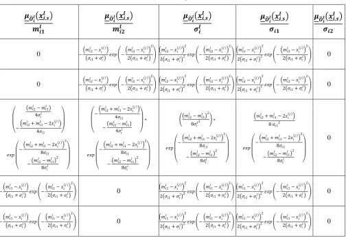
Table II. The derivatives of 𝝁𝑶
𝒊
𝒍 𝒙𝒊,𝒔𝒍 with respect to all 𝜽𝒊,𝒋𝒍
𝝁
𝑶𝒊 𝒍
𝒙
𝒊,𝒔𝒍𝒎
𝒊𝟏𝒍𝝁
𝑶𝒊 𝒍
𝒙
𝒊,𝒔𝒍𝒎
𝒊𝟐𝒍𝝁
𝑶𝒊 𝒍
𝒙
𝒊,𝒔𝒍𝝈
𝒊𝒍𝝁
𝑶𝒊 𝒍
𝒙
𝒊,𝒔𝒍𝝈
𝒊𝟏𝝁
𝑶𝒊 𝒍
𝒙
𝒊,𝒔𝒍𝝈
𝒊𝟐0 − 𝑚𝑖2
𝑙 − 𝑥 𝑖(𝑗 )
𝜎𝑖1+ 𝜎𝑖𝑙
𝑒𝑥𝑝 − 𝑚𝑖2
𝑙 − 𝑥 𝑖(𝑗 )
2
2 𝜎𝑖1+ 𝜎𝑖𝑙
𝑚𝑖2𝑙 − 𝑥 𝑖(𝑗 )
2
2 𝜎𝑖1+ 𝜎𝑖𝑙 2
𝑒𝑥𝑝 − 𝑚𝑖2
𝑙 − 𝑥 𝑖(𝑗 )
2
2 𝜎𝑖1+ 𝜎𝑖𝑙
𝑚𝑖2𝑙 − 𝑥 𝑖 (𝑗) 2
2 𝜎𝑖1+ 𝜎𝑖𝑙 2
𝑒𝑥𝑝 − 𝑚𝑖2
𝑙 − 𝑥 𝑖(𝑗 )
2
2 𝜎𝑖1+ 𝜎𝑖𝑙 0
0 − 𝑚𝑖2
𝑙 − 𝑥 𝑖(𝑗 )
𝜎𝑖1+ 𝜎𝑖𝑙
𝑒𝑥𝑝 − 𝑚𝑖2
𝑙 − 𝑥 𝑖(𝑗 )
2
2 𝜎𝑖1+ 𝜎𝑖𝑙
𝑚𝑖2𝑙 − 𝑥𝑖(𝑗 ) 2
2 𝜎𝑖1+ 𝜎𝑖𝑙
2𝑒𝑥𝑝 −
𝑚𝑖2𝑙 − 𝑥𝑖(𝑗 ) 2
2 𝜎𝑖1+ 𝜎𝑖𝑙
𝑚𝑖2𝑙 − 𝑥𝑖(𝑗) 2
2 𝜎𝑖1+ 𝜎𝑖𝑙
2𝑒𝑥𝑝 −
𝑚𝑖2𝑙 − 𝑥𝑖(𝑗 ) 2
2 𝜎𝑖1+ 𝜎𝑖𝑙
0
𝑚𝑖2𝑙 − 𝑚𝑖1𝑙
4𝜎𝑖𝑙
− 𝑚𝑖2
𝑙 + 𝑚 𝑖1𝑙 − 2𝑥𝑖(𝑗 )
4𝜎𝑖1
𝑒𝑥𝑝 −
𝑚𝑖2𝑙 + 𝑚𝑖1𝑙 − 2𝑥𝑖 𝑗 2
8𝜎𝑖1
− 𝑚𝑖2𝑙 − 𝑚𝑖1𝑙 2
8𝜎𝑖𝑙
− 𝑚𝑖2𝑙 + 𝑚
𝑖1 𝑙 − 2𝑥
𝑖 𝑗
4𝜎𝑖1
− 𝑚𝑖2
𝑙 − 𝑚 𝑖1 𝑙
4𝜎𝑖𝑙
∗
𝑒𝑥𝑝 −
𝑚𝑖2𝑙 + 𝑚𝑖1𝑙 − 2𝑥𝑖 𝑗 2
8𝜎𝑖1
− 𝑚𝑖2𝑙 − 𝑚𝑖1𝑙 2
8𝜎𝑖𝑙
𝑚𝑖2𝑙 − 𝑚𝑖1𝑙 2
8𝜎𝑖𝑙 2 ∗
𝑒𝑥𝑝 −
𝑚𝑖2𝑙 + 𝑚𝑖1𝑙 − 2𝑥𝑖 𝑗 2
8𝜎𝑖1
− 𝑚𝑖2
𝑙 − 𝑚 𝑖1 𝑙 2
8𝜎𝑖𝑙
𝑚𝑖2𝑙 + 𝑚𝑖1𝑙 − 2𝑥𝑖 𝑗
8 𝜎𝑖12
𝑒𝑥𝑝 −
𝑚𝑖2𝑙 + 𝑚𝑖1𝑙 − 2𝑥𝑖 𝑗 2
8𝜎𝑖1
− 𝑚𝑖2𝑙 − 𝑚𝑖1𝑙 2
8𝜎𝑖𝑙
0
− 𝑚𝑖1
𝑙 − 𝑥 𝑖(𝑗 )
𝜎𝑖1+ 𝜎𝑖𝑙
𝑒𝑥𝑝 − 𝑚𝑖1
𝑙 − 𝑥 𝑖(𝑗 )
2
2 𝜎𝑖1+ 𝜎𝑖𝑙 0
𝑚𝑖1𝑙 − 𝑥𝑖(𝑗 ) 2
2 𝜎𝑖1+ 𝜎𝑖𝑙
2𝑒𝑥𝑝 −
𝑚𝑖1𝑙 − 𝑥𝑖(𝑗 ) 2
2 𝜎𝑖1+ 𝜎𝑖𝑙
𝑚𝑖1𝑙 − 𝑥𝑖(𝑗 ) 2
2 𝜎𝑖1+ 𝜎𝑖𝑙
2𝑒𝑥𝑝 −
𝑚𝑖1𝑙 − 𝑥𝑖(𝑗 ) 2
2 𝜎𝑖1+ 𝜎𝑖𝑙 0
− 𝑚𝑖1
𝑙 − 𝑥 𝑖(𝑗 )
𝜎𝑖1+ 𝜎𝑖𝑙
𝑒𝑥𝑝 − 𝑚𝑖1
𝑙 − 𝑥 𝑖(𝑗 )
2
2 𝜎𝑖1+ 𝜎𝑖𝑙
0 𝑚𝑖1
𝑙 − 𝑥 𝑖(𝑗 )
2
2 𝜎𝑖1+ 𝜎𝑖𝑙
2𝑒𝑥𝑝 −
𝑚𝑖1𝑙 − 𝑥𝑖(𝑗 ) 2
2 𝜎𝑖1+ 𝜎𝑖𝑙
𝑚𝑖1𝑙 − 𝑥𝑖(𝑗 ) 2
2 𝜎𝑖1+ 𝜎𝑖𝑙
2𝑒𝑥𝑝 −
𝑚𝑖1𝑙 − 𝑥𝑖(𝑗 ) 2
2 𝜎𝑖1+ 𝜎𝑖𝑙
0
Table III. The derivatives of 𝝁
𝑶𝒊𝒍 𝒙𝒊,𝒔 𝒍
with respect to all𝜽𝒊,𝒋𝒍
𝝁𝑶 𝒊 𝒍 𝒙𝒊,𝒔𝒍
𝒎𝒊𝟏𝒍
𝝁𝑶 𝒊 𝒍 𝒙𝒊,𝒔𝒍
𝒎𝒊𝟐𝒍
𝝁𝑶 𝒊 𝒍 𝒙𝒊,𝒔𝒍
𝝈𝒊𝒍
𝝁𝑶 𝒊 𝒍 𝒙𝒊,𝒔𝒍
𝝈𝒊𝟏
𝝁𝑶 𝒊 𝒍 𝒙𝒊,𝒔𝒍
𝝈𝒊𝟐
− 𝑚𝑖1
𝑙 − 𝑥 𝑖(𝑗 )
𝜎𝑖2+ 𝜎𝑖𝑙
𝑒𝑥𝑝 − 𝑚𝑖1
𝑙 − 𝑥 𝑖 (𝑗 ) 2
2 𝜎𝑖2+ 𝜎𝑖𝑙 0
𝑚𝑖1𝑙 − 𝑥 𝑖 (𝑗 )
2 𝜎𝑖2+ 𝜎𝑖𝑙
2𝑒𝑥𝑝 −
𝑚𝑖1𝑙 − 𝑥 𝑖(𝑗 )
2
2 𝜎𝑖2+ 𝜎𝑖𝑙 0
𝑚𝑖1𝑙 − 𝑥 𝑖 (𝑗 )
2 𝜎𝑖2+ 𝜎𝑖𝑙
2𝑒𝑥𝑝 −
𝑚𝑖1𝑙 − 𝑥 𝑖(𝑗 )
2
2 𝜎𝑖2+ 𝜎𝑖𝑙
0 0 0 0 0
0 0 0 0 0
0 0 0 0 0
0 − 𝑚𝑖2
𝑙 − 𝑥 𝑖(𝑗 )
𝜎𝑖2+ 𝜎𝑖𝑙
𝑒𝑥𝑝 − 𝑚𝑖2
𝑙 − 𝑥 𝑖(𝑗 )
2
2 𝜎𝑖2+ 𝜎𝑖𝑙
𝑚𝑖2𝑙 − 𝑥𝑖(𝑗 ) 2
2 𝜎𝑖2+ 𝜎𝑖𝑙
2𝑒𝑥𝑝 −
𝑚𝑖2𝑙 − 𝑥𝑖(𝑗 ) 2
2 𝜎𝑖2+ 𝜎𝑖𝑙 0
𝑚𝑖2𝑙 − 𝑥𝑖(𝑗 ) 2
2 𝜎𝑖2+ 𝜎𝑖𝑙
2𝑒𝑥𝑝 −
𝑚𝑖2𝑙 − 𝑥𝑖(𝑗 ) 2
[image:11.595.53.545.495.739.2]