Singular Spectrum Analysis: Methodology and Comparison

Munich Personal RePEc Archive

Singular Spectrum Analysis:

Methodology and Comparison

Hassani, Hossein

Cardiff University and Central Bank of the Islamic Republic of Iran

1 April 2007

Online at

https://mpra.ub.uni-muenchen.de/4991/

Singular Spectrum Analysis: Methodology and Comparison

Hossein Hassani

Cardiff University and Central Bank of the Islamic Republic of Iran

Abstract: In recent years Singular Spectrum Analysis (SSA), used as a powerful technique in time series analysis, has been developed and applied to many practical problems. In this paper, the performance of the SSA tech-nique has been considered by applying it to a well-known time series data set, namely, monthly accidental deaths in the USA. The results are com-pared with those obtained using Box-Jenkins SARIMA models, the ARAR algorithm and the Holt-Winter algorithm (as described in Brockwell and Davis (2002)). The results show that the SSA technique gives a much more accurate forecast than the other methods indicated above.

Key words: ARAR algorithm, Box-Jenkins SARIMA models, Holt-Winter algorithm, singular spectrum analysis (SSA), USA monthly accidental deaths series.

1. Introduction

The Singular Spectrum Analysis (SSA) technique is a novel and powerful technique of time series analysis incorporating the elements of classical time series analysis, multivariate statistics, multivariate geometry, dynamical systems and signal processing.

The possible application areas of SSA are diverse: from mathematics and physics to economics and financial mathematics, from meterology and oceanology to social science and market research. Any seemingly complex series with a potential structure could provide another example of a successful application of SSA (Golyandina et al., 2001).

The aim of SSA is to make a decomposition of the original series into the sum of a small number of independent and interpretable components such as a slowly varying trend, oscillatory components and a structureless noise.

of complex trends and periodicities; 7) finding structure in short time series; and 8) change-point detection.

Solving all these problems corresponds to the basic capabilities of SSA. To achieve the above mentioned capabilities of SSA, we do not need to know the parametric model of the considered time series.

The birth of SSA is usually associated with the publication of papers by Broomhead (e.g. Broomhead and King, 1986) while the ideas of SSA were inde-pendently developed in Russia (St. Petersburg, Moscow) and in several groups in the UK and USA. At present, the papers dealing with the methodological aspects and the applications of SSA number several hundred (see, for example, Vautard

et al., 1992; Ghil and Taricco, 1997; Allen and Smith, 1986; Danilov, 1997; Yiou

et al., 2000 and references therein). A thorough description of the theoretical and practical foundations of the SSA technique (with several examples) can be found in Danilov and Zhigljavsky (1997) and Golyandinaet al. (2001). An elementary introduction to the subject can be found in Elsner and Tsonis (1996).

The fact that the original time series must satisfy a linear recurrent formula (LRFs) is an important property of the SSA decomposition. Generally, the SSA method should be applied to time series governed by linear recurrent formulae to forecast the new data points. There are two methods to build confidence intervals based on the SSA technique : the empirical method and the bootstrap method. The empirical confidence intervals are constructed for the entire series, which is assumed to have the same structure in the future. Bootstrap confidence intervals are built for the continuation of the signal which are the main components of the entire series (Golyandina et al., 2001).

Real time series often contain missing data, which prevent analysis and re-duces the precision of the results. There are different SSA-based methods for filling in missing data sets (see, for example, Schoellhamer, 2001; Kondrashovet al., 2005; Golyandina and Osipov, 2006; Kondrashov, 2006).

Change point detection in time series is a method that will find if the struc-ture of the series has changed at some time point by some cause. The method of change-point detection described in Moskvina and Zhigljavsky (2003) is based on the sequential application of SSA to subseries of the original series and moni-tors the quality of the approximation of the other parts of the series by suitable approximates. Also, it must be mentioned that the automatic methods of iden-tification main components of the time series within the SSA framework have been recently developed (see, for example, Alexandrov and Golyandina, 2004a; Alexandrov and Golyandina, 2004b).

with several other methods for forecasting results.

2. Methodology

Consider the real-valued nonzero time series YT = (y1, . . . , yT) of sufficient

length T. The main purpose of SSA is to decompose the original series into a sum of series, so that each component in this sum can be identified as either a trend, periodic or quasi-periodic component (perhaps, amplitude-modulated), or noise. This is followed by a reconstruction the original series.

The SSA technique consist of two complementary stages: decomposition and reconstruction and both of which include two separate steps. At the first stage we decompose the series and at the second stage we reconstruct the original series and use the reconstructed series (which is without noise) for forecasting new data points. Below we provide a brief discussion on the methodology of the SSA technique. In doing so, we mainly follow Golyandina et al. (2001, chap. 1 and 2).

2.1 Stage 1: Decomposition

First step: Embedding

Embedding can be regarded as a mapping that transfers a one-dimensional time series YT = (y1, . . . , yT) into the multi-dimensional seriesX1, . . . , XK with

vectors Xi = (yi, . . . , yi+L−1)

′

∈ RL_{, where K = T −L +1. Vectors X} i are

called L-lagged vectors (or, simply,lagged vectors). The single parameter of the embedding is the window length L, an integer such that 2_≤L _≤T. The result of this step is the trajectory matrixX= [X1, . . . , XK] = (xij)L,Ki,j=1.

Note that the trajectory matrix X is a Hankel matrix, which means that all the elements along the diagonali+j=constare equal. Embedding is a standard procedure in time series analysis. With the embedding performed, future analysis depends on the aim of the investigation.

Second step: Singular value decomposition (SVD)

The second step, the SVD step, makes the singular value decomposition of the trajectory matrix and represents it as a sum of rank-one bi-orthogonal el-ementary matrices. Denote by λ1, . . . , λL the eigenvalues of XX

′

in decreasing order of magnitude (λ1≥. . . λL≥0) and byU1, . . . , UL the orthonormal system

(that is, (Ui, Uj)=0 for i=j (the orthogonality property) andUi=1 (the unit

norm property)) of the eigenvectors of the matrix XX′ corresponding to these eigenvalues. (Ui, Uj) is the inner product of the vectors Ui and Uj and Ui is

the norm of the vector Ui. Set

If we denote Vi = X

′

Ui/

√

λi, then the SVD of the trajectory matrix can be

written as:

X=X1+· · ·+Xd, (2.1)

whereXi=

√

λiUiVi

′

(i= 1, . . . , d). The matricesXi have rank 1; therefore they

are elementary matrices,Ui(in SSA literature they are called ‘factor empirical

or-thogonal functions’ or simply EOFs) andVi (often called ‘principal components’)

stand for the left and right eigenvectors of the trajectory matrix. The collection (√λi, Ui, Vi) is called the i-th eigentriple of the matrix X,

√

λi(i= 1, . . . , d) are

the singular values of the matrix X and the set_{√λi} is called the spectrum of

the matrix X. If all the eigenvalues have multiplicity one, then the expansion (2.1) is uniquely defined.

SVD (2.1) is optimal in the sense that among all the matrices X(r) _{of rank}

r < d, the matrix r_i=1Xi provides the best approximation to the trajectory

matrix X, so that X₋ X(r) _{is minimum. Note that X}2 ₌ d i=1λi

and Xi2 = λi for i = 1, . . . , d. Thus, we can consider the ratio λi/di=1λi

as the characteristic of the contribution of the matrix Xi to expansion (2.1).

Consequently,r_i=1λi/

d

i=1λi, the sum of the firstr ratios, is the characteristic

of the optimal approximation of the trajectory matrix by the matrices of rankr.

2.2 Stage 2: Reconstruction

First step: Grouping

The grouping step corresponds to splitting the elementary matrices Xi into

several groups and summing the matrices within each group. LetI =_{i1, . . . , ip}

be a group of indices i1, . . . , ip. Then the matrixXI corresponding to the group

I is defined as XI=Xi1 +· · ·+Xip. The spilt of the set of indicesJ = 1, . . . , d

into the disjoint subsetsI1, . . . , Im corresponds to the representation

X=XI1 +· · ·+XIm. (2.2)

The procedure of choosing the sets I1, . . . , Im is called the eigentriple grouping.

For given groupI the contribution of the component XI into the expansion (1)

is measured by the share of the corresponding eigenvalues: _i∈Iλi/di=1λi.

Second step: Diagonal averaging

Diagonal averaging transfers each matrix I into a time series, which is an additive component of the initial series YT. If zij stands for an element of a

matrixZ, then the k-th term of the resulting series is obtained by averaging zij

Figure 1: Death series: Monthly accidental deaths in the USA (1973–1978).

Zis the Hankel matrix _HZ, which is the trajectory matrix corresponding to the series obtained as a result of the diagonal averaging. Note that the Hankelization is an optimal procedure in the sense that the matrix_HZis the nearest toZ(with respect to the matrix norm) among all Hankel matrices of the corresponding size (for more information see Golyandinaet al. (2001, chap. 6, sec. 2)). In its turn, the Hankel matrix _HZ uniquely defines the series by relating the value in the diagonals to the values in the series. By applying the Hankelization procedure to all matrix components of (2.2), we obtain another expansion:

X=XI1 +. . .+XIm (2.3)

where XI1 = HX. This is equivalent to the decomposition of the initial series

YT = (y1, . . . , yT) into a sum of m series:

yt= m

k=1

y(_tk) (2.4)

3. Application

3.1 Death series

The Death series shows the monthly accidental deaths in the USA between 1973 and 1978. This data have been used by many authors (see, for example, Brockwell and Davis, 2002) and can be found in many time series data libraries. We apply the SSA technique to this data set to illustrate the capability of the SSA technique to extract trend, oscillation, noise and forecasting. All of the results and figures in the following application are obtained by means of the Caterpillar-SSA 3.30 software 1_{. Figure 1 shows the Death series over period}

1973 to 1978.

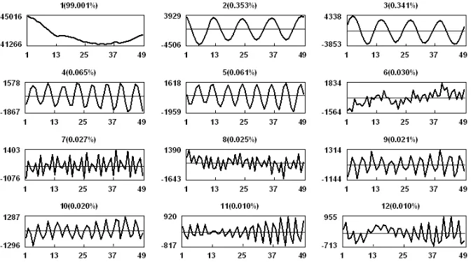
Figure 2: Principal components related to the first 12 eigentriples.

3.2 Decomposition: Window length and SVD

As we mentioned earlier, the window length L is the only parameter in the decomposition stage. Selection of the proper window length depends on the prob-lem in hand and on preliminarily information about the time series. Theoretical results tell us that Lshould be large enough but not greater thanT /2. Further-more, if we know that the time series may have a periodic component with an integer period (for example, if this component is a seasonal component), then to get better separability of this periodic component it is advisable to take the window length proportional to that period. Using these recommendations, we

take L= 24. So, based on this window length and on the SVD of the trajectory matrix (24_×24), we have 24 eigentriples, ordered by their contribution (share) in the decomposition.

Note that the rows and columns of the trajectory matrixXare subseries of the original time series. Therefore, the left eigenvectors Ui and principal components

Vi (right eigenvectors) also have a temporal structure and hence can also be

regarded as time series. Let us consider the result of the SVD step. Figure 2 represents the principal components related to the first 12 eigentriples.

3.3 Supplementary information

Let us describe some information, which proves to be very helpful in the identification of the eigentriples of the SVD of the trajectory matrix of the original series. Supplementary information help us to make the proper groups to extract the trend, harmonic components and noise. So, supplementary information can be considered as a bridge between the decomposition and reconstruction step:

Decomposition_−→Supplementary information_−→Reconstruction

Below, we briefly explain some methods, which are useful in the separation of the signal component from noise.

Auxiliary Information

The availability of auxiliary information in many practical situations increase the ability to build the proper model. Certainly, auxiliary information about the initial series always makes the situation clearer and helps in choosing the parameters of the models. Not only can this information help us to select the proper group, but it is also useful for forecasting and the change point detection based on the SSA technique. For example, the assumption that there is an annual periodicity in the Death series suggests that we must pay attention to the frequency k/12 (k = 1, ...,12). Obviously we can use the auxiliary information to select the proper window length as well.

Singular values

Usually every harmonic component with a different frequency produces two eigentriples with close singular values (except for frequency 0.5 which provides one eigentriples with saw-tooth singular vector). It will be clearer if N,L and K

are sufficiently large.

singular values.

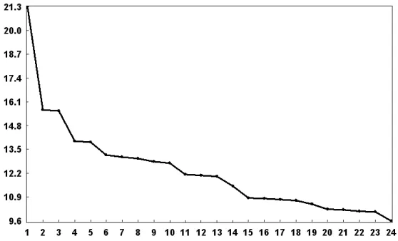
Therefore, explicit plateaux in the eigenvalue spectra prompts the ordinal numbers of the paired eigentriples. Figure 3 depicts the plot of the logarithms of the 24 singular values for the Death series.

Figure 3: Logarithms of the 24 eigenvalues.

Five evident pairs with almost equal leading singular values, correspond to five (almost) harmonic components of the Death series: eigentriple pairs 2-3 , 4-5, 7-8, 9-10 and 11-12 are related to harmonics with specific periods (we show later that they correspond to periods 12, 6, 2.5, 4 and 3).

Pairwise scatterplots

In practice, the singular values of the two eigentriples of a harmonic series are often very close to each other, and this fact simplifies the visual identification of the harmonic components. An analysis of the pairwise scatterplots of the singular vectors allows one to visually identify those eigentriples that corresponds to the harmonic components of the series, provided these components are separable from the residual component.

frequencyw =m/n < 0.5 with relatively prime integer m and n, the points are the vertices of the scatterplots of the regularn-vertex polygon. Figure 4 depicts scatterplots of the 6 pairs of sine/cose sequence (without noise) with zero phase, the same amplitude and periods 12, 6, 4, 3, 2.5 and 2.4.

Figure 4: Scatterplots of the 6 pairs of sines/cosines.

Figure 5 depicts scatterplots of the paired eigenvectors in the Death series, corresponding to the harmonics with periods 12, 6, 4, 3 and 2.5. They are ordered by their contribution (share) in the SVD step.

Figure 5: Scatterplots of the paired harmonic eigenvectors.

Figure 6: periodograms of the paired eigentriples (2–3, 4–5, 7–8, 9–10, 11–12).

Periodogram analysis

considered. We must then look for the eigentriples whose frequencies coincide with the frequencies of the original series.

If the periodograms of the eigenvector have sharp spark around some frequen-cies, then the corresponding eigentriples must be regarded as those related to the signal component.

Figure 6 depicts the periodogram of the paired eigentriples (2–3, 4–5, 7–8, 9–10, 11–12). The information arising from Figure 6 confirms that the above mentioned eigentriples correspond to the periods 12,6,2.5,4 and 3 which must be regarded as selected eigentriples in the grouping step with another eigentriple we need to reconstruct the series.

Separability

The main concept in studying SSA properties is ‘separability’, which char-acterizes how well different components can be separated from each other. SSA decomposition of the series YT can only be successful if the resulting additive

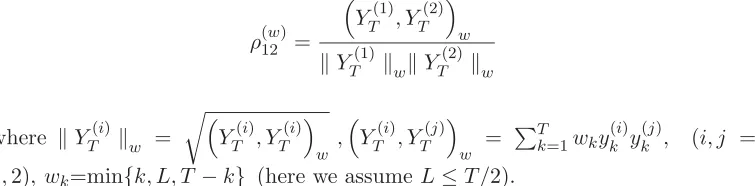
components of the series are approximately separable from each other. The fol-lowing quantity (called the weighted correlation or w-correlation) is a natural measure of dependence between two series Y_T(1) andY_T(2):

ρ(₁₂w)=

Y_T(1), Y_T(2)

w

Y_T(1) _wY_T(2) _w

where Y_T(i)_w = Y_T(i), Y_T(i)

w ,

Y_T(i), Y_T(j)

w =

T

k=1wky( i)

k y

(j)

k , (i, j =

1,2), wk=min{k, L, T −k} (here we assumeL≤T /2).

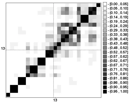
A natural hint for grouping is the matrix of the absolute values of the w -correlations, corresponding to the full decomposition (in this decomposition each group corresponds to only one matrix component of the SVD). If the absolute value of the w-correlations is small, then the corresponding series are almost w -orthogonal, but, if it is large, then the two series are far from beingw-orthogonal and are therefore badly separable. So, if two reconstructed components have zero

w-correlation it means that these two components are separable. Large values of w-correlations between reconstructed components indicate that the compo-nents should possibly be gathered into one group and correspond to the same component in SSA decomposition.

Figure 7: Matrix ofw-correlations for the 24 reconstructed components.

3.4 Reconstruction: Grouping and diagonal averaging

Reconstruction is the second stage of the SSA technique. As mentioned above, this stage includes two separate steps: grouping (identifying signal component and noise) and diagonal averaging (using grouped eigentriples to reconstruct the new series without noise). Usually, the leading eigentriple describes the general tendency of the series. Since in most cases the eigentriples with small shares are related to the noise component of the series, we need to identify the set of leading eigentriples.

Grouping: Trend, harmonics and noise

Trend identification:

Trend is the slowly varying component of a time series which does not contain oscillatory components. Assume that the time series itself is such a component alone. Practice shows that in this case, one or more of the leading eigenvectors will be slowly varying as well. We know that eigenvectors have (in general) the same form as the corresponding components of the initial time series. Thus we should find slowly varying eigenvectors. It can be done by considering one-dimensional plots of the eigenvectors (see, Figure 2).

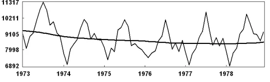
Figure 9 shows the extracted trend which is obtained from the first and sixth eigentriples. It appears that taking the first and sixth eigentriples show the gen-eral tendency of the Death series better than the first eigentriple alone. However, the sixth eigentriple does not completely belong to the trend component but we can consider it as a mixture of the trend and the harmonic component.

Figure 8: Trend extraction (first eigentriple).

Figure 9: Trend extraction (first and sixth eigentriples).

Harmonic identification:

The general problem here is the identification and separation of the oscillatory components of the series that do not constitute parts of the trend. The statement of the problem in SSA is specified mostly by the model-free nature of the method. The choice L = 24 allows us to simultaneously extract all the seasonal com-ponents (12, 6, 4, 3, and 2.5 month) as well as the trend. Figure 10 shows the oscillation of our series which is obtained by the eigentriples 2-12.

Figure 10: Oscillation extraction(eigentriples 2–12).

Figure 11: Oscillation extraction(eigentriples 2–5,7–12).

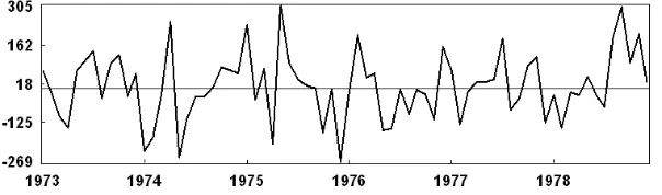
Noise detection:

The problem of finding a refined structure of a series by SSA is equivalent to the identification of the eigentriples of the SVD of the trajectory matrix of this series, which correspond to trend, various oscillatory components, and noise. From the practical point of view, a natural way of noise extraction is the group-ing of the eigentriples, which do not seemgroup-ingly contain elements of trend and oscillations. Let us discuss the eigentriple 13. We consider it as an eigentriple which belongs to noise because the period of the component reconstructed by eigentriple 13 is a mixture of the periods 3, 10, 14 and 24, as the periodogram indicates this cannot be interpreted in the context of seasonality for this series. We will thus classify eigentriple 13 as a part of the noise. Figure 12 shows the residuals which are obtained by the eigentriples 13–24.

Diagonal averaging

The last step of the SSA technique is diagonal averaging. Diagonal averaging applied to a resultant matrix XIk (which is obtained from the grouping step for

the k–th group of m) produces the Yk

T = (y1k, . . . ,ykT) and therefore the initial

series YT = (y1, . . . , yT) is decomposed into the sum of m series yt = mk=1ykt

(1_≤t_≤T).

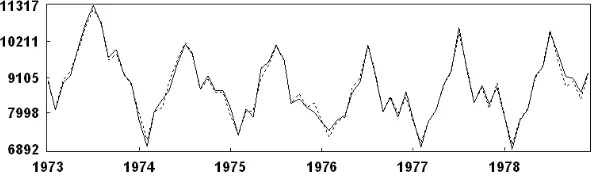
If we just consider the trend (eigentriple 1 or (1 and 6)), harmonic component (eigentriple 2–12 or (2–5, 7–12)) and noise (eigentriple 13–24) as groups then we have 3 groups (m = 3). However we can have 8 groups if we consider each group by detail such as; eigentriples 1, 2–3, 4–5, 6, 7–8, 9-10, 11–12 (which correspond to the signal) and 13–24 or 7 groups if we merge the eigentriples 1 and 6 into a group. Figure 13 shows the result of the signal extraction or reconstruction series without noise which is obtained from the eigentriples 1–12. The dotted and the solid line correspond to the reconstructed series and the original series respectively. As indicated on this figure, the considered groups for the reconstruction of the original series is optimal (bear in mind that the SVD step has optimal properties). If we add the series of Figures 8 and 9 (or 9 and 11) we will obtain the refined series (Figure 13).

Figure 13: Reconstructed series (eigentriples 1–12).

3.5 Forecasting

Forecasting by SSA can be applied to time series that approximately satisfy linear recurrent formulae (LRF).

We shall say that the seriesYT satisfies an LRF of orderdif there are numbers

a1, . . . , ad such that

yi+d= d

k=1

akyi+d−k, 1≤i≤T −d.

un-der term-by-term addition and multiplication. LRFs are also important for prac-tical implication. To find the coefficients a1, . . . , ad we can use the eigenvectors

obtained from the SVD step or characteristic polynomial (for more information see Golyandina et al. (2001, chap. 2 and 5)).

Assume that we have a series YT =Y_T(1)+Y_T(2)and the problem of forecasting

its componentY_T(1). IfY_T(2)can be regarded as noise, then the problem is that of forecasting the signalY_T(1) in the presence of a noiseY_T(2). The main assumptions are:

(a) the seriesY_T(1) admits a recurrent continuation with the help of an LRF of a relatively small dimension d, and

(b) there exists a numberL such that the seriesY_T(1) and Y_T(2) are approximately separable for the window length L.

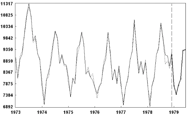
Figure 14 shows the original series (solid line), reconstructed series (dotted line) and its forecasting after 1978 (the six data points of 1979). The vertical dotted line shows the truncation between the last point of the original series and the forecast starting point. Figure 14 shows that the reconstructed series (which is obtained from eigentriples 1-12) and the original series are close together indicating that the forecasted values are reasonably accurate.

Figure 14: Original series (solid line), reconstructed series (dotted line) and the 6 forecasted data points of 1979.

4. Comparison

and the Seasonal Holt-Winters Algorithm. Brockwell and Davis (2002) applied these methods on the Death series to forecast the six future data points. Be-low, these methods are described shortly and the results of their forecasting are compared with the SSA technique.

SARIMA model

Box and Jenkins (1970) provide a methodology for fitting a model to an empirical series. This systematic approach identifies a class of models appropriate for the empirical data sequence at hand and estimates its parameters. A general class of Box and Jenkins models includes ARIMA and SARIMA models that can model a large class of autocorrelation functions. We use the models below for forecasting the six future data as are described in Brockwell and Davis (2002): Model I:

∇12yt= 28.831 + (1−0.478B)(1−0.588B12)Zt ;

Model II:

∇12yt= 28.831 +Zt−0.596Zt−1−0.407Zt−6−0.685Zt−12+ 0.460Zt−13,

where Zt∼W N(0,94390) and the backward shift operatorB is: BjZt=Zt−j.

ARAR algorithm

The ARAR algorithm is an adaption of ARARMA algorithm (Newton and Parzen, 1984) in which the idea is to apply automatically selected ‘memory-shortening’ transformations (if necessary) to the data and then to fit an ARMA model to the transformed series. The ARAR algorithm used here is a version of this in which the ARMA fitting step is replaced by the fitting of the subset AR model to the transformed data.

Holt-Winter eeasonal algorithm (HWS)

Results

Table 1 shows the results for several methods for the forecasting of the six future data points. To calculate the precision we have used two measures, namely, the Mean Absolute Error (MAE) and the Mean Relative Absolute Error (MRAE). This table shows that the forecasted values are very close to the original data for the SSA technique. We borrow the result of forecasting for the other methods from Brockwell and Davis (2002, chap. 9). The methods are arranged based on the performance of forecasting. The values MAE and MRAE show the performance of forecasting (the value of the MRAE is rounded). As it appears in Table 1, the SSA technique is the best among the methods considered, for example, the value of MAE or MRAE for the SSA methods is 3 times less than the first one (model I) and 2 times less than the HWS algorithm.

Table 1: Forecast data, MAE and MRAE for six forecasted data by several methods.

1 2 3 4 5 6 MAE MRAE

Original Data 7798 7406 8363 8460 9217 9316

Model I 8441 7704 8549 8885 9843 10279 524 6 % Model II 8345 7619 8356 8742 9795 10179 415 5 % HWS 8039 7077 7750 7941 8824 9329 351 4 % ARAR 8168 7196 7982 8284 9144 9465 227 3 % SSA 7782 7428 7804 8081 9302 9333 180 2 %

Note that by using the above mentioned information and the SSA-Caterpillar software, anyone can repeat the results presented in this paper for each part such as the results of the forecasting in Table 1.

5. Conclusion

Acknowledgement

The author gratefully acknowledges Professor A. Zhigljavsky for his encour-agement, useful comments and helpful technical suggestions that led to the im-provement of this paper. The author would also like to thank the Central Bank of the Islamic Republic of Iran for its support during his research study at Cardiff University.

References

Alexandrov, Th. and Golyandina, N. (2004). The automatic extraction of time series trend and periodical components with the help of the Caterpillar SSA approach.

Exponenta Pro3-4, 54-61.(In Russian.)

Alexandrov, Th. and Golyandina, N. (2004). Thresholds setting for automatic extrac-tion of time series trend and periodical components with the help of the Caterpillar SSA approach. Proc. IV International Conference SICPRO’05, 25-28.

Allen, M. R. and Smith, L. A. (1996). Monte Carlo SSA: Detecting irregular oscillations in the presence of coloured noise. Journal of Climate 9, 3373-3404.

Box, G. E .P. and Jenkins, G. M. (1970). Time Series Analysis: Forecasting and Control, Holden-Day.

Brockwell, P. J. and Davis, R. A. (2002). Introduction to Time Series and Forecasting, 2nd edition. Springer.

Broomhead, D. S. and King, G. P. (1986). Extracting qualitative dynamics from ex-perimental data. Physica D 20, 217-236.

Danilov, D. (1997). Principal components in time series forecast. Journal of Computa-tional and Graphical Statistics 6, 112-121.

Danilov, D. and Zhigljavsky, A. (Eds.). (1997). Principal Components of Time Series: the ‘Caterpillar’ method, University of St. Petersburg Press. (In Russian.) Elsner, J. B. and Tsonis, A. A. (1996). Singular Spectral Analysis. A New Tool in Time

Series Analysis. Plenum Press.

Ghil, M. and Taricco, C. (1997). Advanced spectral analysis methods. In Past and present Variability of the Solar-Terrestrial system: Measurement, Data Analysis and Theoretical Model (Edited by G. C. Castagnoli and A. Provenzale), 137-159. IOS Press.

Golyandina, N., Nekrutkin, V. and Zhigljavsky, A. (2001). Analysis of Time Series Structure: SSA and related techniques. Chapman & Hall/CRC.

Kondrashov, D. and Ghil1, M. (2006). Spatio-temporal filling of missing points in geophysical data sets. Nonlin. Processes Geophys 13, 151-159.

Kondrashov, D., Feliks, Y. and Ghil, M. (2005). Oscillatory modes of extended Nile

River records (A. D. 622–922),Geophys. Res. Lett32, L10702, doi:10.1029/2004GL022156. Moskvina, V. G. and Zhigljavsky, A. (2003). An algorithm based on singular spectrum

analysis for change-point detection. Communication in Statistics - Simulation and Computation32, 319-352.

Newton, H. J. and Parzen, E. (1984). Forecasting and time series model types of eco-nomic time series. In Major Time Series Methods and Their Relative Accuracy

(Edited by S. Makridakis,et al.), 267-287, Wiley.

Schoellhamer, D. H. (2001). Singular spectrum analysis for time series with missing data. Geophys. Res. Lett28, 3187-3190.

Vautard, R., Yiou, P. and Ghil, M. (1992). Singular-spectrum analysis: A toolkit for short, noisy chaotic signal. Physica D58, 95-126.

Yiou, P., Sornette, D. and Gill, M. (2000). Data-adaptive wavelets and multi-scale singular spectrum analysis. Physica D142, 254-290.

Received November 3 1, 2006; accepted March 2, 2007.

Hossein Hassani Group of Statistics

Cardiff School of Mathematics Cardiff University

Senghennydd Road Cardiff CF24 4AG, UK [email protected]

and also at

2- Central Bank of the Islamic Republic of Iran 207/1, Pasdaran Avenue