Algorithm for Optimum Sizing of a Photovoltaic Water
Pumping System
Imene Yahyaoui
Dept. Systems Engineering and Automatic
Industrial Eng. School Valladolid, Spain
Mahmoud Ammous
Dept. Electric Engineering National School of Engineeing
Sfax, Tunisia
Fernando Tadeo
Dept. Systems Engineering and Automatic
Industrial Eng. School Valladolid, Spain
ABSTRACT
A sizing algorithm for a photovoltaic water pumping installation composed of photovoltaic panels, battery’ bank, DC/AC converters and a water pump is presented. Considering criteria related to the battery’ bank safe operation, fulfilling the water volume needed by the crops and ensuring a continuous operation of the pump, the algorithm decides the size of the installation’ components. The installation’ cost using the presented and the basic algorithms are compared. Obtained results confirm that the water demand is covered during the crops’ vegetative cycle with a minimum use of the battery’ bank and minimum cost.
General Terms
Sizing, Photovoltaic Energy.Keywords
Photovoltaic energy, sizing algorithm, water, pumping.
1.
INTRODUCTION
The need to save water and energy is a serious issue that has increased in importance over the last years and will become more important in the near future [1]. The low price of fuel is the reason why renewable energy sources are not used in several applications, including water pumping. So, pumping systems based on renewable energies are still scarce, even though it has clear advantages, namely, low generating costs, suitability for remote areas, and being environmentally friendly. Nowadays, the price of electric energy is rising constantly, and water and energy companies are investing in more efficient solutions [2].
Renewable Energies have been used in water pump applications, especially in remote agricultural areas, thanks to the potential of renewable energies. The renewable energies’ use depends on the user’s propensity to invest in renewable based pumping systems, his/her awareness and knowledge of the technology for water pumping, and also on the availability, reliability, and economics of conventional options [3]. Moreover, the evaluation of the groundwater volume required for irrigation and its availability in the area is also relevant in determining the profitability of using renewable energies.
Some installations combine solar panels and wind turbines to compensate the solar radiation and the wind velocity fluctuations. These sources act in a complementary way, since, generally, when the solar radiation is high, the wind velocity is low. This combination may result in a more reliable but complex water pumping, since electric power generated by wind turbines is highly erratic and may affect both the power quality and the planning of power systems [4]. Hence, there is a multitude of systems based on renewable
pump’ supply depends essentially on the site characteristics and the water needed by the crops. As Tunisia’s climate is considered semi-arid and it is good insolated country [5], the use of a photovoltaic autonomous installation for water pumping in remote areas is required. Thus, since the sizes of the photovoltaic installation components affect its autonomy [6, 7], it is necessary to define some adequate values for the components’ parameters, such as the photovoltaic panel surface and the number of batteries [8, 9].
the water volume needed for tomatoes’ irrigating, the site characteristics, the solar radiation and the photovoltaic panel type, the proposed algorithm provides the optimum values of the panel surface and the number of batteries. Indeed, the idea consists in calculating the values that guarantee, on the one hand, the balance between the charged and discharged energy in the battery’ bank, and on the other hand, the pumping of the water volume needed. It is important to point out that the components size chosen must fulfill the irrigation requirements for all the months of the tomatoes’ vegetative cycle (March to July). In this paper, the algorithm is developed and validated using measured meteorological data. Moreover, an economic comparison between the proposed and the basic sizing methods is presented. The models used for the panels and the batteries are summarized in section 2. The sizing algorithm is proposed in section 3. The algorithm’ results are summarized in section 4. Finally, the conclusion is presented in section 5.
2.
SYSTEM COMPONENTS’
MODELING
In order to size and control the system elements, an essential step consists in modeling the installation components. Hence, some models for the photovoltaic panels, the batteries and the pump are presented now.
2.1
Photovoltaic Panel Model
A yield based panel model is used to model the photovoltaic values (the temperature coefficient for the panel yield, the module [17, 20]. This yield is evaluated using the cell parameters panel yield at the reference temperature, etc.), and the cell temperature module, which depends on the Nominal Operating Cell Temperature (NOCT) and the clearness index [20]. This model is given by
:
( ) (1- ( ( ) - )) pv t r pv T tc Tref
(1)
where: r is the panel yield at the reference temperature,pv is the temperature coefficient for the panel yield (C1),
( )
c
T t is the cell temperature (ºC), Tref is the reference temperature (°C).
The cell temperature T tc( ) is calculated using [20]:
- T( ) ( ) ,
800 ref
c a t
NOCT
T t T t H t d (2)
where Ta is the ambient temperature (°C), H t,dt
is the solar radiation on the tilted panel (W/ m2), NOCT is the Normal Operating Cell Temperature (ºC).The photovoltaic power is evaluated using [20]:
( ) ,
pv t pv
P t S H t d t (3)
where S is the panel surface (m2).
2.2
Battery Bank Model
A non-linear model for modeling the lead- acid battery is used [66]. In addition to its simplicity, this model has the advantage of using the battery current to describe precisely the battery behavior when charging or discharging. Its performance is then evaluated from its capacity Cp and its depth of discharge dod.
The stored charge in the battery CR is described by [17]:
-1 3600 p ( k ) ( k ) ( k )
k
R R bat
k
C C I (4)
where k is the time between instant k1and k and kp is the Peukert.
The depth of discharge dod is given by [17, 20]:
1 R k
k
p C dod
C
(5)
Fig. 1. Scheme of the off-grid photovoltaic irrigation system
where Cp is the Peukert capacity, considered constant (A.h).
2.3
Pump
As in most research related to water pumping, the motor pump adopted is an induction machine (IM), thanks to the simplicity of control and the encouraging price [17]. The total mechanical power on the shaft coupled to the pump PL is [17]:
h L
p
V g H
P
t
(6)
where V is the pumped water volume (m3),g is the gravity acceleration (m/s2), is the water density (Kg/m3), Hh is the head height (m), p is the pump efficiency, t is the
3.
ALGORITHM PROPOSAL
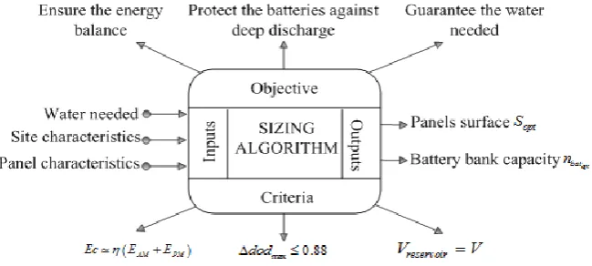
A good sizing must fulfill that the installation provide the electrical demand of the load [17]. Hence, the proposed algorithm’s main objective is to ensure the load supply throughout the day, while protecting the battery’ bank against deep discharge or excessive charge and guaranteeing the water volume needed for the crops’ irrigation. The scheme of the proposed approach is presented in Fig. 2 [19]. The algorithm depends on:
the water volume needed,
the site characteristics,
the panel characteristics,
The algorithm aims to find the optimum panels’ surface Sopt and the batteries’ number
opt
bat
n that guarantee the installation’ autonomy when supplying the pump. Hence, the idea consists in searching the optimal components sizes that ensure the balance between the charged and the extracted energies Ec and Ee, respectively. In fact, the battery bank supply the load when the panels do not generate the sufficient power, and is charged with the PV energy produced in excess (Fig. 3). The energy balance can be expressed by:
c AM PM
E ; E E (7)
The sizing algorithm is performed using two sub algorithms during the crops’ vegetative cycle (March to July): the first Algorithm 2.1 allows the size of the panel surface SM and
the number of batteries
M
bat
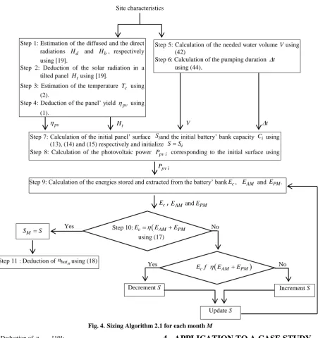
n to be determined for each month M. Then, Algorithm 2.2 is performed to deduce the final system components’ sizes. Algorithm 2.1 is detailednow in steps following the approach presented in Fig. 4.
a) Algorithm 2.1: Determination of SM and
M
bat
n
Step 1 Estimation of the diffused and direct radiation [19]. Step 2 Deduction of the solar radiation H t,dt
in a tiltedpanel [19].
Step 3 Estimation of the cell temperature T tc
using (2). Step 4 Deduction of the panel yield pv
t using (1) [17]. Step 5 Calculation of the crops’ water needs V: The [image:3.595.134.458.415.746.2]determination of the water volume needed for tomato growth is essential to define the amount of water to be pumped. The water volume depends essentially on the crop growth stage and the evapotranspiration [19]. In the literature, many models have been used to describe the evapotranspiration. For instance, [19] used the Penman Method, which depends essentially on the net radiation at the crop surface, the mean air temperature, and the wind speed. [19] presented some models to describe the evapotranspiration, such as the Thorenthwet method, which depends on the sunlight duration and the air temperature. The Blaney-Criddle method has also been used.
Fig. 2. Planning of the proposed sizing algorithm
Time (h)
P
o
w
er
(
W
)
P
pv Ppump
EA M EPM
[image:3.595.134.459.417.563.2]This method includes the seasonal crop coefficient kc, in addition to the sunlight duration and the air temperature, which provides better patterns of the needed water volume. For this reason, the Blaney-Criddle method is used.
The daily water volume, Vn, required by the crop is given by [19]:
n c To
V k E (8)
where kc is the monthly crop growth coefficient, ETo is the monthly reference evapotranspiration average, which depends on the ratio of the mean daily daytime hours for a given month to the total daytime hours in the year p and the mean monthly air temperature T for the corresponding month, is evaluated [19]:
0 46 8 13
To
E K p . T . (9)
where K is the correction factor, expressed by [19]: 0 03 0 24
K . T .
To obtain the necessary gross water, it is essential to estimate the irrigation losses. For this, an additional water quantity must be provided for the irrigation to compensate for those losses. Thus, the final water volume is evaluated by [19]:
1
1
11
i R
c To m
i R
f L
V k E r
f L
(10)
where: rm is the the average monthly rain volume, fi is the leaching efficiency coefficient as a function of the irrigation water applied [19], LR is the leaching fraction given by the humidity that remains in the soil, expressed by [19]:
5
-w R
e w
EC L
EC EC
(11)
w
EC is the electrical conductivity of the irrigation water (dS.
-1
m ) and ECeis the crop salt tolerance (dS. m-1).
Step 6 Calculation of the pumping duration t. In the application, the pump’s flux is constant. Thus, t can be evaluated by (12):
pump P t
Q
(12)
Step 7 Calculation of the minimum panel surface Si, Smax and the initial battery capacity Ci using equations (13), (14) and (15) respectively, based on the irrigation frequency [20].
For March and April,
2
aut pump
rech i
pv bat l pv reg d
P t
d S
W
(13)
For May, June and July,
2 1
pump aut
i
rech pv bat l pv reg
P t d
S
d
W
(14)
d aut
i
bat max
E d C
V dod
(15)
with Ppumpis the pump power (W), t is the water pumping duration (h), daut is the days of autonomy,
rech
d is the days needed to recharge the battery, Wpv is the average daily radiation (Wh/m2/ day), batis the electrical efficiency of the battery bank, l is the electrical efficiency of the installation, pv is the efficiency of each photovoltaic panel, reg is the regulator performance, Ed is the the daily consumption (W.h), Vbat is the battery voltage (V),
max dod
is the the maximum dod variation (%). Step 8 Calculation of Ppvi corresponding to the minimum
panel surface Si, using (16) [19]: pv i pv i t
P S H (16)
where npvis the panels’ yield (%), Ht is the solar radiation on a tilted panel (W/ m2), Siis the initial panel surface (m2),
Step 9 Calculation of the energies expected to be stored and extracted from the battery each day by evaluating the area Ec and Ee, respectively, (Fig. 3).
If the discharged energy is higher than the charged energy, the algorithm increases the panel surface by the minimum increment of the PVP size commercially available: the algorithm looks for the best configuration to guarantee the balance between the demanded and the produced energies, by ensuring the equality between the charged Ec and discharged energies Ee in the battery bank (7).
Step 10The balance between the accumulated and the extracted energies does not guarantee the system’s autonomy, due to the fluctuation in the solar radiation and the energy losses in the installation’ components. Thus, to ensure the system’s autonomy and protect the battery against deep discharges, the algorithm is performed by adopting an efficiency coefficient that allows the dod to be less than dodmax ( is equal to 1.14*
error
). Thus, equation (7) becomes:
c AM PM
Fig. 4.Sizing Algorithm 2.1 for each month M
Step 11 Deduction of
M
bat
n [19]:
M
c bat
bat
E n
C
(18)
where Ecis the energy charged in the battery bank (Wh) and
bat
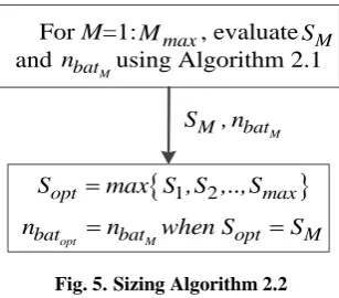
C is the nominal capacity for one battery (Ah), b) Algorithm 2.2: Deduction of Sopt and
opt
bat n
Using Algorithm 2.2, presented in Fig. 5, the final values of the panel surface Sopt and the capacities number
opt
bat
n , are then deduced. Sopt corresponds to the maximum value of the panel surface obtained during the months. The optimum batteries number is the corresponding value for Sopt, since it is the most critical month.
4.
APPLICATION TO A CASE STUDY
The proposed algorithm is tested during the months that correspond to the vegetative cycle of tomatoes (March to July), using data of the target area. Algorithm 2.1 is first evaluated. In fact, the solar radiation accumulated on a tilted panel is evaluated [19]. Then, the panel yield is calculated for each month using (1) (Table 1). In parallel, the water needed V is calculated, depending on the crops vegetative cycle and the site characteristics using (10). The initial values Si, and Ci are summarized in Table 2, and used to test the condition presented in (17). Indeed, if the charged energy is higher than the discharged energy, the panel surface is increased by the minimum panel available surface in the market ( the increment is 0.5m2), and vice versa.Site characteristics
Step 1: Estimation of the diffused and the direct radiations Hd and Hb, respectively using [19].
Step 2: Deduction of the solar radiation in a tilted panel Htusing [19].
Step 3: Estimation of the temperature Tc using (2).
Step 4: Deduction of the panel’ yield pv using (1).
Step 5: Calculation of the needed water volume V using (42)
Step 6: Calculation of the pumping duration t using (44).
pv
Ht
Step 7: Calculation of the initial panel’ surface and the initial battery’ bank capacity using (13), (14) and (15) respectively and initialize .
Step 8: Calculation of the photovoltaic power Ppv i corresponding to the initial surface using (16).
i
S Ci
i SS
V t
pv i P
Step 9: Calculation of the energies stored and extracted from the battery’ bank , and . Ec EAM EPM
c
E
,
EAM andEPM
c AM PM
E E E
Step 10:
using (17) Yes
M
S S
Step 11 : Deduction of using (18) nbatM
c AM PM
E f E E
No
Decrement S
Yes No
Increment S
26
For
M
=1: , evaluate
and using Algorithm 2.1
MS
M
bat
n
max
M
1 2
opt max
S
max S ,S ,..,S
opt M
bat bat opt M
n
n
when S
S
M
M bat
[image:6.595.89.243.71.206.2]S
, n
Fig. 5.Sizing Algorithm 2.2
Algorithm 2.1 results are summarized in Table 3 and Fig. 6-7. They show that the proposed algorithm always ensures the needed water volume, respects the battery bank’ depth of discharge limits and the energy balance. In fact, in Fig. 6 the proposed algorithm guarantees the needed water volume for the crops irrigation, since the pump is supplied by the panels and the battery bank. This has been proved for March to July (Fig. 7). Moreover, this algorithm ensures the energy balance for each month M. For example, in Table 3, the efficiency coefficient is around the fixed value (1=1.26) throughout all the considered months. For this value, dodis guaranteed to be equal to 0.88. Thus, the extracted energy
Ee is almostequal to the accumulated energy (Ec). For instance, in March, the generated photovoltaic power during the morning is used to supply the pump together with the battery bank during the pumping duration. Then, the photovoltaic power generated is used to charge the batteries for the rest of the day hours. The quotient between the cumulated and extracted energies is equal to 1.29, which is near to the value initially fixed in Algorithm 2.1
1 26.
. For July, the error coefficient is fixed to be 66.67 %Hence, the obtained panels’ surface Sopt and the batteries number
opt
bat
n satisfy the energy balance. In other terms, all the stored energy is consumed, thanks to the batteries number calculation, which is done by considering the same maximum
max
dod
value for all the months (dodmax= 0.88). Hence,
[image:6.595.318.540.74.325.2]the panels’ surface allows the load to be supplied during the pumping duration and provides the energy needed to charge the batteries (Fig. 8).
Fig.6. Evaluation of Algorithm 2.1 for each month using mean climatic data values
Fig.7. Daily energies using mean climatic data values for each month M using algorithm 2.1
Table 1 Panel efficiency calculation and irrigationparameters estimation
March April May June July
pv
W (W.h) 8094.0 10254.0 11197.0 12974 12077
pv
(%) 12.37 12.21 11.90 11.50 11.17
Water volume m /3 10ha 60.70 100.37 179.82 241.10 321.03
Pumping duration t
(h) 2.51 4.14 7.42 9.95 13.25
2 14
0 5 10 15 20 25 30
En
erg
y
(k
W
h
)
2 14
0.5 1 1.5 2
Ec
/E E
e
E c E e E c /E e
March June July
1.26
May April
Months
4 6 8 10 12 14 16 18 20 22
0 0.2 0.4 0.6 0.8 1
dod
4 6 8 10 12 14 16 18 20 22
0 5 10 15 20 25
Ppvst Pmpp Ppump kW
Results
March April May June July
W
(W.h) (23) 8094.0 10254.0 11197.0 12974 12077July, M=5
July, M=5
Time (h)
Months
[image:6.595.318.540.365.516.2] [image:6.595.100.497.581.728.2]Table 2 Initial values of the panels’ surface and number of batteries
March April May June July
Initial panel surface ( 2
m )
11 27.5 92 108.5 156.5
Initial batteries numbers
i
C
11 5 9 12 16
Table 3 Calculation of the minimum panel surface and the batteries’ number needed to fulfill the energy requests each month M
March April May June July
error
(%) 90 90 90 90 66.67AM PM
E
E
(W.h) 11100.0 13606.0 11232.0 11511.0 15450.0c
E
(W.h) 14347 17882.0 14499.0 14572.0 26018.0pump
E
(W.h) 11278 18648.0 33409.0 44796.0 59040.0PV
E
(W.h) 16034 25122 40488 52741 81822
2M
S
m
17.5 23 31.5 40 68M
bat
n
6 7 6 6 131
c
AM PM
E
E
E
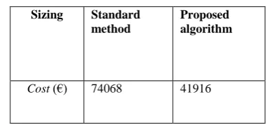
1.29 1.31 1.29 1.27 1.68To demonstrate the efficiency of the proposed algorithm from an economic point of view, a brief economic comparison is now presented. Hence, the installation’ cost (19) is evaluated, using the components sizes obtained by the proposed and the standard sizing methods [21] (table. 4):
1
1 1 1
1
pv pv y pv bat b b b y b b
chop chop chop chop chop y chop inv inv
inv y inv
Cost n C n M n C y C n y M
n C y n M n y C y
M n y
(19)
Table 4 Cost evaluation of the PV installation
Sizing Standard method
Proposed algorithm
Cost (€) 74068 41916
where npvis the number of photovoltaic modules and nbat is the batteries number
Results
March April May June July
pv
W
(W.h) (23) 8094.0 10254.0 11197.0 12974 12077pv
(%) (25) 12.37 12.21 11.90 11.50 11.17Water volume
3
10
m /
ha
(42) 60.70 100.37 179.82 241.10 321.03Pumping duration
t
(h) (44) 2.51 4.14 7.42 9.95 13.25Results
[image:7.595.328.526.550.641.2]Fig.8. Evaluation of the algorithm 2.2 using measured data for July
5.
CONCLUSIONS
An algorithm to decide on the components sizing of a pumping installation is proposed and tested for a 10 ha land surface in the Northern of Tunisia. The algorithm ensures the system’s autonomy, the batteries safe operation and the needed water volume for irrigation. A cost comparison between the basic and the proposed sizing methods proves that the proposed algorithm allows the installation’ cost to be decreased.
6.
ACKNOWLEDGMENTS
Miss Yahyaoui is supported by a grant from MICInn BES-2011-047807.
7.
REFERENCES
[1] Gaikwad, D. D., Chavan, M. S. 2015. A Novel Algorithm for MPPT for PV Application System by use of Direct Control Method. International Journal of Computer Applications. (2015), 10-15.
[2] Ramos, J. S., Ramos, H. M. 2009. Sustainable application of renewable sources in water pumping systems: Optimized energy system configuration. Energy Policy. (2009), 633-643.
[3] Sree Manju, B., Ramaprabha, R., Mathur, B.L. 2011. Design and Modeling of Standalone Solar Photovoltaic. International Journal of Computer Applications. (2011), 41-45.
[4] Díaz-González, F., Sumper, A., Gomis-Bellmunt, O., Villafáfila-Robles, R. 2012. A review of energy storage technologies for wind power applications. Renewable and Sustainable Energy Reviews. (2012), 2154-2171. [5] Rana, G., Katerji, N., Lazzara, P., Ferrara, R. M. 2012.
Operational determination of daily actual evapotranspiration of irrigated tomato crops under Mediterranean conditions by one-step and two-step models: Multiannual and local evaluations. Agricultural Water Management. (2012), 285-296.
[6] Kaldellis, J. K., Zafirakis, D., Kondili, E. 2010. Optimum sizing of photovoltaic-energy storage systems for autonomous small islands. International Journal of Electrical Power & Energy Systems. (2010), 24-36. [7] Sidrach-de-Cardona, M., Mora López, L. 1998. A simple
model for sizing stand-alone photovoltaic systems. Solar Energy Materials and Solar Cells. (2010), 199-214. [8] Eteiba, M. B. A., El Shenawy, E. T., Shazly, J. H.,
Hafez, A. Z. 2013. Photovoltaic (Cell, Module, Array) Simulation and Monitoring Model using MATLAB®/GUI Interface. International Journal of Computer Applications. (2013), 69, 14-28.
[9] Jakhrani, A. Q., Othman, A.K., Rigit, A., Ragai. H., Samo, S. R., Kamboh, S. A. 2012. A novel analytical model for optimal sizing of standalone photovoltaic systems. Energy. (2012), 675-682.
[10] Acakpovi, A., Xavier, F. F., Awuah-Baffour, R. 2012. Analytical method of sizing photovoltaic water pumping system. In the proceedings of the 4th IEEE International Conference on Adaptive Science & Technology, 65-69. [11] Shrestha, G. B., Goel, L. 1998. A study on optimal sizing
of stand-alone photovoltaic stations. IEEE Transactions on Energy Conversion. (1998), 373-378.
[12] Barra, L., Catalanotti, S., Fontana, F., Lavorante, F. 1984. An analytical method to determine the optimal size of a photovoltaic plant. Solar Energy. (1984), 509-514. [13] Groumpos, P. P., Papageorgiou, G. 1987. An optimal
sizing method for stand-alone photovoltaic power systems. Solar Energy.(1987), 341-351.
[14] Mellit, A., Benghanem, M., Hadj Arab, A., Guessoum, A. 2003. Modelling of sizing the photovoltaic system parameters using artificial neural network. In the proceedings of the IEEE Conference on Control Applications, 353-357.
[15] Yang, H., Zhou, W., Lu, L., Fang, Z. 2008. Optimal sizing method for stand-alone hybrid solar–wind system with LPSP technology by using genetic algorithm. Solar Energy. (2008), 354-367.
[16] Mellit, A., Benghanem, M., Kalogirou, S. A. 2007. Modeling and simulation of a stand-alone photovoltaic system using an adaptive artificial neural network: Proposition for a new sizing procedure. Renewable Energy. (2077), 285-313.
[17] Ben Ammar, M. 2011. Contribution à l’optimisation de la gestion des systèmes multi-sources d’énergies renouvelables. Thesis presented at the National School of Engineering of Sfax, Tunisia.
[18] Bernal-Agustín, J. L., Dufo-López, R. 2009. Simulation and optimization of stand-alone hybrid renewable energy systems. Renewable and Sustainable Energy Reviews. (2009), 2111-2118.
[19] Yahyaoui, I., Chaabene, M., Tadeo, F. 2013. An algorithm for sizing photovoltaic pumping systems for tomato irrigation. In the proceedings of the IEEE Conference on Renewable Energy Research and Applications (ICRERA). (2013), 1089-1095.
[20] Chaabene, M. 2009. Gestion énergétique des systèmes photovoltaïques. A master course at the National School of Engineering of Sfax, Tunisia, (2009).
[21] Eftichios, K., Dionissia. K., Antonis, P., Kostas, K. 2006. Methodology for optimal sizing of stand-alone photovoltaic/wind-generator systems using genetic algorithms. Solar energy. (2006), 1072-1088.
4 6 8 10 12 14 16 18 20 22
0 0.2 0.4 0.6 0.8 1
dod
Time (h)
4 6 8 10 12 14 16 18 20 22
0 2 4 6 8 10
Time (h)
Pmpp Ppump
kW July, M=5