Munich Personal RePEc Archive
Chaos in the tourism industry
Correani, Luca and Garofalo, Giuseppe
University of Tuscia in Viterbo - Department Distateq
2008
Online at
https://mpra.ub.uni-muenchen.de/9677/
Chaos in the tourism industry
Luca Correani, Giuseppe Garofalo
July 22, 2008
Abstract
The paper presents an application of the chaos theory to tourism, a sector in which operators’ choices are particularly elaborate and complex. The dynamics of the tourist industry are, in fact, the result of close inter-actions between units of production, tourist flows, local authorities and natural resources. These interactions do not necessarily lead to a regular trend in the development of the tourist industry as proposed by Butler; on the contrary, irregularities of various types are very possible. The model microfounds rigorously on both the demand and the supply side. Firms and tourists operate under the hypothesis of limited rationality, the former in an oligopolistic context, the latter on the basis of mechanisms of evolu-tionary selection. Although not exhaustive, the model forms a theoretical platform that can be easily adapted to hypotheses and situations that differ from those originally hypothesized. As a consequence, this paper presents a series of numerical simulations. The results show the chaotic nature of a tourist flow, which limits the practicability of measures intro-duced to stabilise the system. In their place, measures are needed that stimulate a continuous reshaping of the system in relation to the factors that tend to change it. JEL classification: C73, L10, L83, Q01
Keywords: sustainable tourism, chaos, evolutionary games
1
Introduction
The theory of the life cycle of tourist destinations proposed by Butler (1980) is still at the centre of intense scientific debate today. Even though it is recog-nised by scholars as the reference framework for the study of the dynamics of the tourist industry, Butler’s approach does not account for the frequent differ-ences to be found between the time series of tourist flows and their theoretical
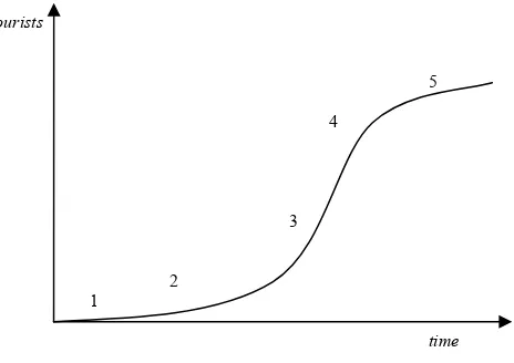
forecasts. The life cycle follows a regular succession of five stages,exploration,
involvement,development,consolidationandstagnation(Figure 1), followed by
believe that the theory of the post-stagnation stages needs to be revised (Agar-wal, 1997; Priestley-Mundet, 1998; Aguil`o-Alegre-Sard, 2005).
time tourists
1
2
3 4
[image:3.595.179.411.188.352.2]5
Figure 1: Butler’s cycle - 1) Exploration 2) Involvement 3) Development 4)Consolidation 5)
Stagnation.
The general view that emerges from the numerous empirical tests carried out is that Butler’s model has to be considered primarily as descriptive rather than normative (Haywood, 1986; Cooper-Jackson, 1989; Ioannides, 1992; Opperman, 1995, Hovinen, 1981, 2002). Certainly there are some studies that reveal a signif-icant correlation between time series and the theoretical model (see for example Meyer-Arendt, 1985; Douglas, 1997), but they are to be considered as one of the many possible manifestations of the development of a tourist locality. One of the main limitations of the model is that it does not explicitly consider the effects of factors, both external and internal to the system, on the evolutionary dynamics of the tourist industry under examination: variations in the number of firms working in the sector, the preferences of tourists, competition or the quality of the environment can generate substantial changes in the normal de-velopment of a tourist destination. For example, Lundtorp-Wanhill (2001) show how, when assessing the nature of tourist flows from the habitual to the occa-sional, substantial changes can be seen in the regularity of the cycle as proposed
by Butler, so much so as to make the authors define it as a ”caricature” of the
real situation.
during the long life cycle of many tourist localities (Russell, Faulkner, 1999; Prideaux, 2000; Hovinen, 2002; Zahra, Ryan, 2007), but this requires a com-plete re-conceptualisation of the theory that integrates research on tourism with other scientific sectors, such as environmental economics, ecology and the theory of complexity (Farrel, Twining-Ward, 2004). An interesting theoretical model that has moved in this direction is the one proposed by Casagrandi-Rinaldi (2002). Their description of a tourist system is based on the interaction of three fundamental elements, tourist flow, environment and capital, described by a system of differential equations. A study of the system reveals the presence of points of bifurcation at which significant changes in the behaviour of the system
can be observed with minimal variations in the reference parameters 1.
Al-though this model provides interesting suggestions for analysis, it nevertheless lacks a rigorous microfoundation of the equations that describe the system: in particular, it does not explain the mechanisms that regulate the decision-making processes of a tourist. The same fault can be found in the model proposed by Hernandez-Leon (2007), which is very similar to the one that has just been described. Once again the fundamental equations of the system, even though they are able to reproduce the dynamics of Butler’s cycle, are not the result of a rigorous formalization of the behaviour of the agents involved.
The model presented in this paper starts from these points and attempts to describe the evolutionary dynamics of a hypothetical tourist industry through the interaction of demand (tourist flow), supply (oligopolistic firms) and natural environment, but also introduces some new aspects that can be summarised in four points:
1. the tourist industry is assumed to be made up of a certain number of local firms (destinations), each one organised in a Cournot framework of symmetrical oligopoly. The formal situation of oligopoly means that the quantity of services produced and the price charged can be calculated for each locality in each period. The choice of an oligopolistic form of the market is logical if we consider that there is a limited number of firms in a local industry, that entry is expensive and that there exists a high degree of substitutability between the tourist services offered by the firms. This last point justifies the symmetry of oligopoly. Two levels of competition are considered in the model: the first concerns firms in the same locality and therefore in competition with each other, whilst the second involves different localities competing to gain an ever larger share of the tourist population;
2. the tourist flow towards a locality is regulated by the level of surplus obtained on average by the tourist that decides to visit it: this surplus depends on both the level of the services in the industry and the quality of the environment. The mathematical law that formalises the dynamics of a tourist flow draws on the replicator theory (Taylor-Jonker, 1978; Weibull, 1998), which can often be found in evolutionary game theory. In sum-marising the decision-making processes of a tourist, it takes into account not only the surplus that can be obtained in the different localities, but also factors such as popularity and congestion, all in a non deterministic
1A similar analysis applied to the interaction between collective actions and the use of
context. Choice will also depend on the probability of acquiring informa-tion about the localities. This informainforma-tion is acquired through random exchanges about the experiences of single tourists. The use of the evolu-tionary approach makes it possible to implicitly consider a more realistic and limited rationality of tourists; in fact, in a world characterised by scarce information a tourist will not necessarily choose the destination that guarantees the greatest surplus.
Papatheodorou (2005) formalises a tourist’s choice as if he were perfectly rational, informed and maximising his own utility function. Although it is a well-established approach and can be easily applied, we have preferred to adopt what, in our opinion, is a more realistic selection model, in which the tourist has little information about the different tourist destinations and limited rationality, in the sense that he can continue to prefer localities that guarantee lower levels of surplus;
3. the mathematical law that describes the dynamics of a tourist flow is unknown to firms, which therefore find that they have to optimize their profits period by period, as they cannot plan a path for the efficient de-velopment of production and tourism in advance. We believe that this approach to be truer to the real situation and in any case closer to the spirit of the model developed here, which aims to investigate the chaotic aspects of the system rather than define the deterministic laws that are valid in the long run;
4. the model has been developed in discrete time. The time unit chosen refers to the time necessary for the tourist industry to significantly change its production apparatus and therefore the quantity of services produced. The assumption is that the tourist industry changes its capacity slowly; even if individual firms can change their production of tourist services within a short period of time, we believe that the overall impact on the system is negligible and only after a fairly long period can a relevant change be observed. Furthermore, this choice of method is essential, given the fact that, unlike differential equations, difference equations obtained in a model with discrete time can generate chaotic dynamics if they take
on specific mathematical forms2.
In addition to productive activities and the movement of tourists, the model also tries to highlight the deterioration and recovery of the quality of the environ-ment which characterises the developenviron-ment phases of the tourist locality, in order to assess environmental sustainability. The structure of the model provides for the tourist flow to be distributed among different localities (oligopolies), thus affecting the quality of the environment in each one, both directly through the pollution produced by each tourist and indirectly by stimulating the production of services. The levels of production and the quality of the environment, in turn, condition the dynamics of the tourist flow by changing its distribution.
As we were unable to trace the general properties of the model to test whether the model structured in this way is capable of reproducing both reg-ular Butler-type dynamics and chaotic trajectories, and thus to explain the
2It is well known in the literature how the logistic equationx
complexity of the evolutionary processes observed in many tourist localities, we preferred to use the method of numerical simulations and limit the study to only two competing tourist localities. We assumed the system is in an initial state of equilibrium, in which only one of the two destinations is fully developed. We then concentrated our attention on the less developed locality and studied the processes of growth in relation to changes in the parameters of the model.
Even though it is not exhaustive, the picture that emerges from the study of the bifurcation diagrams enables us to make some important observations about the complexity of the evolutionary dynamics of the tourist industry and
the role of policy measures3. In particular, the scenarios that emerge from the
simulations suggest the following observations:
1. Significant changes in the state of the system can be induced by variations that concern one or more of the following factors: elasticity of demand, tourist preferences, costs of production, number of firms and the environ-mental impact of the tourist industry;
2. As McKercher (1999) maintained, both linear and non linear processes are active in tourist systems; the prevalence of one or the other depends on the phase in which the system is at a certain moment. The tourist flow can therefore appear stable, or at least evolve in a regular and predictable way, for long periods and then suddenly become chaotic. The simulations have in fact reproduced this type of behaviour of tourist flows fairly consistently, thus showing how the initial Butler-type phases of development can be followed by markedly unstable, typically cyclical or chaotic dynamics;
3. The more or less stable nature of the dynamics is strongly influenced by factors that can be traced back mainly to consumer tastes, sensibility to price and, to a certain extent, unforeseeable events such as environmental disasters and political instability. The model focuses mainly on the first two factors, leaving
to one side the role played by catastrophic events4
Although the model proposed here does not consider all the factors that play a role in the development of a tourist industry (for example, it does not consider transport costs), it nevertheless forms a valid theoretical platform. Further extensions and elaborations may be introduced, with particular reference to the mechanisms of interaction between the industrial organisation of the production system and the decision-making of the tourist.
3We were guided in our choice of analysis techniques by an interesting article by
Currie-Kubin (2006), in which the use of bifurcation diagrams helped to highlight the chaotic nature of the dynamics generated inCore-Periphery models, thus seriously questioning all the basic assumptions of ’New Economic Geography’.
4The inclusion of catastrophic factors would have meant considering some stochastic
dis-turbance; this approach, however, would go against the basic idea of the model which is to reproduce endogenously chaotic dynamics without the intervention of exogenous shocks. For a discussion of the management of catastrophic events in the tourist industry, see Ritchie (2004). In particular the inconstancy of tourists can produce significant changes in both the level of demand elasticity and the criteria followed in the selection of the localities to visit, thus generating strong and unforeseeable fluctuations in tourist flows;
The paper is structured in three parts: in the first, the mathematical struc-ture of the model is developed to obtain the basic equation that describes the dynamics of a tourist flow; the second part presents the results of the numer-ical simulations and the analysis of the bifurcation diagrams; the third part concludes by discussing the possible developments and extensions of the model.
2
The Model
2.1
Tourists
The tourist flow towards a given locality is generally regulated by its popularity and by the average level of satisfaction obtained by those who choose to visit it. The positive assessment attributed to the locality by a tourist will be communi-cated to other potential tourists who, with a certain degree of probability, will then decide to spend their holidays at that destination. The level of probability tends to increase, the greater the popularity of the tourist destination and the degree of satisfaction reached by the visitors, whereas it decreases as the level of popularity and satisfaction of other competing localities increases.
Consider a set i∈D of tourist localities competing to attract ever greater
shares of tourists by attracting them away from other competing localities. The
potential population of tourists is exogenous and equal toMmax, whilstmi,t
in-dicates the share of tourists that at timetchooses destinationi, for a total
num-ber of tourists equal toMi,t =mi,tMmax. The vector mt=m1,t, ..., mi,t, ...
describes, therefore, the state of the tourist population at timet.
A tourist compares his experience at timetwith that of another tourist
cho-sen at random from the population. The exchange of information can force him, with a certain probability, to review his preferences and choose a different local-ity for the following period. If both tourists have had the same experience, that
is, at time tthey visited the same locality, they will not obtain any additional
information and so they have no incentive to change tourist destination. The only element that distinguishes one tourist from another, therefore, is the different experiences they have acquired by visiting different localities in the same period. We rule out the possibility that the two tourists can have different
opinions about the same locality they have visited5.
Given the constancy of the tourist population, it is assumed implicitly that the tourist has an infinite life or that, once information is obtained, he is sub-stituted by a perfect copy of himself (descendent), to whom all the information acquired will be transferred (which means, for the purposes of the results, ex-actly the same thing). It will be the descendent at that point to decide whether
to return to the old destination or go to a new one6. From this moment onwards,
for the sake of simplicity, we assume that the tourist lives eternally and therefore
5Further extensions of the model could take into account a certain heterogeneity in the
assessments of tourists who have had the same experiences, by distinguishing, for example, mass tourism from ecotourism. This hypothesis, however, would require a subdivision of the tourist population into at least two subpopulations and the identification of an evolutionary mechanism that explains the prevalence of one type of tourism over the other, thus making the model much more complex.
6The model also allows for the fact that a tourist can acquire information from other
there will be no need to continuously distinguish between the descendent and the parent.
It is well to point out that the experience of a tourist is limited to the
knowledge of the characteristics of the two localities: the one visited at timet
and the one that he decides to visit at timet+ 1. The experiences before time
t have therefore been forgotten.
LetPt(Vi→Vj|Tk) withi, j, k∈Dbe the probability that a tourist, visiting
localityiat timetdecides to visit localityjin the following period, on the basis
of the information received at time tby a tourist in localityk.
Having assumed that a tourist considers the possibility of changing
desti-nation from i to j, only after having exchanged opinions with someone who
has already visited the other locality, we can write thatPt(Vi→Vj|Tk) = 1 if
i =j = k andPt(Vi→Vj|Tk) = 0 if k=i 6=j or k =6 i, k6= j, i6=j. If the
comparison was made with someone with the same experience, the tourist (or likewise his direct descendent) will return to the old destination with probability equal to 1; similarly, the probability that he decides to visit a different locality without having had information from a tourist who has already been there is zero.
In other cases in which i 6= k, j =k or i = j 6= k, the law of conditional
probability Pt(Vi →Vj|Tk) =Pt(Vi→Vj, Tk)/Pt(Tk)>0 stands.
If we consider localityiwe can determine its net tourist flow by finding the
difference between the number of tourists arriving and leaving in a certain pe-riod of time. On the basis of the assumed imitative process, the flow of tourists
arriving is equal toP
k∈D,k6=imk,tMmaxPt(Vk →Vi, Ti) whilst those leaving is
P
k∈D,k6=imi,tMmaxPt(Vi→Vk, Tk), from which we obtain the dynamic
equa-tion for the tourist flow:
mi,t+1−mi,t =
X
k∈D,k6=i
mk,tPt(Vk→Vi|Ti)Pt(Ti) +
−mi,tPt(Vi→Vk|Tk)Pt(Tk) (1)
wherePt(Th) =mh,t ∀h∈D.
The exchange of information between tourists mainly concerns their level of satisfaction and the popularity of the destination they visited. And therefore it is reasonable to suppose that the conditional probability, that is, the probability of changing destination once the information has been obtained from another tourist, will depend exactly on these factors, that is:
Pt(Vk →Vi|Ti) =fk(Sck,t, Sci,t, mi,t, mk,t) ,
Pt(Vk →Vk|Ti) = 1−fk(Sck,t, Sci,t, mi,t, mk,t)
with ∂fk/∂Sck,t < 0, ∂fk/∂Sci,t > 0, ∂fk/∂mk,t > 0, ∂fk/∂mi,t < 0,
0≤fk≤1, ∀k6=i∈D.
Let us indicate withSci,tandSck,tthe utility (surplus) obtained on average
in time t from tourists in localities i and k, whose popularity is measured by
As suggested by Weibull (1998), it is assumed that the conditional probabil-ity to reach a localprobabil-ity in the following period is proportional to the popularprobabil-ity of that locality and that the factor of proportionality is positively correlated with the present surplus that can be obtained in the same locality. By indicating
withωk(Sci,t)>0 the factor of proportionality that the tourist inkassociates
with localityi, we can write
Pt(Vk→Vi|Ti) = ωk(Sci,tω)km(i,tSc+i,tω)km(Sci,tk,t)mk,t Pt(Vk→Vk|Ti) = ωk(Sci,tω)km(Sci,tk,t+ω)km(Sck,tk,t)mk,t
with∂ωk/∂Sci,t >0 ∀i, k∈D.
By substituting in [1] we obtain the basic equation of the model
mi,t+1=mi,t+
X
k∈D,k6=i
mk,t
ωk(Sci,t)mi,t
ωk(Sci,t)mi,t+ωk(Sck,t)mk,t
mi,t+
−mi,t
ωi(Sck,t)mk,t
ωi(Sci,t)mi,t+ωi(Sck,t)mk,t
mk,t (2)
from which it only remains to specify the exact form of the factors of
propor-tionalityωand its surplus, which are given in paragraphs 3 and 2.2 respectively.
2.2
Firms
Each locality of set D represents a tourist industry which is assumed to be
structured as a Cournot-type oligopoly with homogeneous firms7. The term
’in-dustry’ should not be understood as the whole tourist system in a country, but the set of firms in a certain locality whose organisation, geographical position and environmental resources can be considered a system in itself and which has certain characteristics that distinguish it from other tourist localities (indus-tries) (the classic example is an island that attracts tourists during the summer
period)8. The group of firms belonging to each of the tourist destinations is
considered exogenous and is indicated byN ={Nd}d∈D.
Each firm belonging to localityd chooses at time t the quantity of tourist
services to be produced and supplied, in order to maximise the following profit function in that period:
Πd,i,t=P
PNd
j=1qd,j,t, Md,t, Ed,t
qd,i,t−cdqd,i,t,
7The hypothesis that the tourist industry is organised along the lines of oligopolistic
com-petition has been analysed by Davies (1999) and Baum-Mudambi (1995). For a review, see Davies and Dawnward (2005).
8It is necessary to point out that the dynamics of a tourist industry are not neutral in
with∀i= (1, ..., Nd),∀d∈D whereP(.) indicates the inverse demand function
that depends on the total quantity of services produced by the tourist industry
PNd
j=1qd,j,t, on the flow of tourists arrivingMd,t and on the level of
environmen-tal qualityEd,t, whilstcdis the same marginal cost for all the firms in the same
industry9.
The greater the flow of tourists and the better the quality of the
environ-ment, the higher the price per unit of tourist service, that is ∂P/∂Md,t > 0
and ∂P/∂Ed,t > 0. If we assume that the inverse demand function is pt =
Md,t(Ed,t+ 1)/PNj=1d qd,j,t
ǫd
, with 1/ǫd>1 to indicate the (constant) price
elasticity of demand, and consider the symmetrical nature of oligopoly, we
ob-tain the quantity of tourist services produced by firmiat timet
q∗
d,i,t=qd,t∗ =
Md,t(Ed,t+ 1)
Nd
N
d−ǫd cdNd
1/ǫd ,
withNd> ǫd ∀d∈D.
If we substitute the equilibrium quantity in the inverse demand function we
obtain the equilibrium price p∗ = Nd−ǫd
cdNd
−1
which depends entirely on the structural parameters of the local industry. A fixed factor, equal to 1, is added to the value of the quality of the environment in order to avoid the cessation of all productive activities, if it is annulled. It is correct, in fact, to assume that a tourist locality can continue to exist even in the presence of a very degraded natural environment, as in the case of mass tourism which is very often attracted to the wide range of entertainment facilities on offer rather than to the natural beauty of a place.
By integrating the demand function, the average surplusScd,t obtained by
a tourist who visits localitydat timetis:
Scd,t= 1
Md,t
Z ∞
p∗
Md,t(Ed,t+ 1)
p1/ǫd d,t
dp= (Ed,t+ 1) ǫd
1−ǫd
Nd−ǫd
cdNd
1−ǫd
ǫd .
Given that a tourist flow towards a certain locality is also affected by the surplus obtained in other localities, the model presents two types of strategic interaction: one between firms in the same locality and the other between com-peting tourist destinations. But, whereas in the first the quantity of tourist services produced by firms in the same industry acts as an element of reciprocal conditioning, the second works through variations in the surplus and therefore
in the flows of tourists that go to the different localities10.
9Firms act under the assumption of bounded rationality as they do not know the law of
motion of tourist flow (2). This hypothesis, as well as being realistic, also simplifies somewhat the calculations. If this had not been so, we would, in fact, have had to solve the complex problem of inter-temporal optimization in a differential game (oligopoly). For an application of this type, see Candela-Cellini (2004).
10A possible extension of the model could be that the profits of firms in a certain
lo-cality were also dependent on the quantity of services produced in other competing des-tinations, thus introducing a further factor of strategic interaction between local tourist industries. In this case the demand function would assume the following form: pt =
“
Md,t
`
Ed,t+ 1
´
/“PNd
j=1qd,j,t+
P
g∈D,g6=d
PNg
i=1qj,i,t
””ǫd
2.3
The natural environment
The production of services and the flow of tourists have an immediate impact on the quality of the environment. By indicating the maximum possible level
for the quality of the environment in localitydwith ˆEd , that is, the level that
would be reached in the absence of a tourist industry, the quality of the
envi-ronment at timetis expressed by the following expression:
Ed,t=max
n
ˆ
Ed−αMd,t−βNdqd,t∗ ,0
o
,
withα >0 andβ >0 to indicate the impact of tourist flows and the production
of tourist services on the environment respectively. Once the quality of the environment has been lost, it can only be recovered by reducing production or the number of tourists. Natural resources used by the industry are not renewable so long as the source of pollution persists in the territory: therefore, once the quality of the environment has been destroyed, it can be recovered only by reducing the number of tourists and production.
The natural environment is considered as a fixed stock of environmental re-sources localised in a specific territory. This can be left in its original state, by guaranteeing the natural wealth that is present, or it can be allocated to an economic use, by establishing infrastructures for tourism with a consequent
reduction in its quality. By substituting inq∗
d,t and solving the equation forEd,t
we obtain
Ed,t=max
ˆ
Ed−Md,t
α+βNd−ǫd
cdNd
1/ǫd
1 +βMd,t
Nd−ǫd cdNd
1/ǫd ,0
,
from which the maximum limit of sustainable tourism can be calculated, that is, the share of the tourist population which corresponds to quality zero of the environment:
ˆ
md=
ˆ
Ed
Mmax·
α+βNd−ǫd
cdNd
1/ǫd,
withEd,t= 0 ∀md,t>mˆd.
The limit ˆmdis therefore a specific factor of a locality which is determined by
the combination of environmental factors ( ˆEd, α, β), structural components of
the industry (Nd, cd) and elements connected with the psychology of the tourist
(ǫd).
At this point a tourist industry can be defined as sustainable if it combines a positive level of environmental quality with a positive flow of visitors, that is,
if it is capable of satisfying both the following conditionsmd,t>0 andEd,t >0
∀t, d∈ D at the same time. Given that the trajectories of a tourist flow can
1. if the orbit of the tourist flow converges on the fixed pointm∗the industry
is sustainable on condition that 0< m∗<mˆ.
2. if the orbit attractor is aPcycle in periodn,P ≡ {mj,mj+1, . . . ,mj+n−1:
g(mj+n−1) =mj}, then the industry is perfectly sustainable on condition
thatEd,t >0∀md,t∈P. There may also be cycles that alternate phases
of total environmental exploitation with phases of a partial recovery of the quality of the environment in a general alternation between environmental sustainability and unsustainability. The same can be said about the orbits which have a chaotic character, but are limited to an interval of values
(mmin, mmax) ; in this case the industry is perfectly sustainable in terms
of the environment if ˆmd > mmax, unsustainable if ˆmd < mmin, whilst
if ˆmd ∈(mmin, mmax) there will be periods of sustainability followed by
phases of total exploitation of the environment.
The possible alternation between environmental sustainability and unsus-tainability can be explained by the fact that a single period of time, taken as the temporal unit of reference in the model, is not completed in a single tourist season, but is considered to be sufficiently long (that is, a number of tourist seasons) to allow an appropriate adaptation of both the quantity of services supplied made by the firms and the recovery of part of the natural environment
that has been destroyed11.
3
The Simulations
A simulation of the model requires an explicit formalization of the factors of proportionality used in the definition of conditional probability.
As in Weibull (1998), let us suppose that ωk(Sci,t) = exp(σ·Sci,t) with
σ≥0. This specification is sufficiently general, because different choice models
can be adopted by the tourist according to the value of the parameterσ:
1. if σ → 0, tourists tend to prefer the most popular tourist locality
inde-pendently of the real benefits that can be obtained;
2. if σ → ∞, tourists tend to choose the tourist locality that guarantees a
higher level of surplus independently of its popularity.
As in fact
Pt(Vk →Vi|Ti) = exp(σ·Sci,texp)m(σi,t·Sc+expi,t)m(σi,t·Sck,t)mk,t,
we have
limσ→0Pt(Vk→Vi|Ti) = mi,tm+i,tmk,t
11On the other hand, the existence of cyclical dynamics in natural capital has been widely
limσ→∞Pt(Vk→Vi|Ti) =
0 ifSck,t> Sci,t
1 ifSck,t< Sci,t
Similar specifications about the probability of a tourist’s choice can be found in Papathodorou (2005) and Morley (1994).
Let us assume that there are two localities, that isD={A, B}, in order to
make the study of the model simpler without compromising the purpose of the analysis, which is to identify the chaotic behaviours of a tourist flow in a system
of interacting tourist industries12. This does not prevent us from considering
industry A as a single industry, whilst B is the set of tourist industries in
competition with it, that is to say B = {B1, ...., Bn}. On the basis of this
specification the conditional probabilities are
Pt(VA→VB|TB) =fA= e
σ·ScB,t(1−m A,t) eσ·ScB,t(1−m
A,t)+eσ·ScA,tmA,t
Pt(VB →VA|TA) =fB= e
σ·ScA,tmA,t
eσ·ScB,t(1−mA,t)+eσ·ScA,tmA,t
Pt(VA→VA|TB) = 1−fA
Pt(VB →VB|TA) = 1−fA
which, substituted in [2], make it possible to obtain the basic equation of the model in an explicit form in relation to the tourist flow that concerns
destina-tionA:
mA,t+1=mA,t+mA,t(1−mA,t)
eσ·ScA,tm
A,t−eσ·ScB,t(1−mA,t) eσ·ScA,tm
A,t+eσ·ScB,t(1−mA,t)
(3)
where formA,t∈[0,1] alsomA,t+1 =g(mA,t)∈[0,1], that isg: [0,1]→[0,1].
The reduction to two tourist industries makes it possible to limit the analysis to the study of the dynamics of the tourist flow of just one industry since, the
dynamics of destination B is determined by the residue, asmB,t= 1−mA,t.
Given the initial statemA,0, the orbit of the system is unequivocally defined.
The first iteration ismA,1=g(mA,0), the secondmA,2=g(mA,1) =g(g(mA,0))
12Remember that, in addition to competition between industries which determines the
and so on. By indicating the n-th iteration byg[n](m
A,0) we can represent the
orbit by the vector (mA,0,g(mA,0),g[2](mA,0),g[3](mA,0), . . . ,g[n](mA,0), . . . ),
which in a more compact form becomes
g[n](m
A,0) :n≥0 withg[0](mA,0) =
mA,0. Ifg(m∗) =m∗ then the system is in stationary equilibrium andm∗ is a
fixed point. In the same way, ifg[k]( ˆm) = ˆmthen ˆmis a periodic point and the
orbit
g[n]( ˆm) :n≥0 is periodic in period k. An orbit is defined as chaotic if it
is limited, not periodic and shows a marked sensitivity to the initial conditions, in the sense that, following arbitrarily small variations in these conditions, there are significant changes in the course of the orbit itself.
The functiong(mA,t) has the following fixed points: mA,t = 0, mA,t = 1
and ∀mA,t ∈(0,1) so that eσ·ScA,tmA,t =eσ·ScB,t(1−mA,t). In general there
is no guarantee that a solution mA,t exists that satisfies this condition. In
the particular case of perfect structural homogeneity among tourist localities, which occurs when two destinations have the same parameter values but not necessarily similar levels of development, the system has at least three fixed
points: m∗
A = 0, m∗A = 1 andm∗A = 0.5. Furthermore, in this case if a fixed
point ¯mA∈(0,1) exists with ¯mA6= 0.5, then 1−m¯A is also a fixed point in the
system.
If, in fact,eσ·ScA( ¯mA)m¯
A−eσ·ScB(1−m¯A)(1−m¯A) = 0, from the
hypothe-sis of structural homogeneity we have that ScA(1−m¯A) =ScB(1−m¯A) and
ScA( ¯mA) =ScB( ¯mA), and therefore alsoeσ·ScA(1−m¯A)(1−m¯A)−eσ·ScB( ¯mA)m¯A=
0.
Independently of the degree of structural similarity between the tourist
local-ities, the fixed internal points cannot be analytically determined because mA,t
cannot be made explicit from the condition eσ·ScA,tm
A,t =eσ·ScB,t(1−mA,t).
It is therefore necessary to proceed with the study of the model through
numer-ical simulations on the computer13. They do not provide a detailed study of
the general properties of the model, but highlight how, even in a deterministic context, significant changes in the dynamics of a tourist flow can be generated after minimal variations in the parameters. These changes make it very diffi-cult to predict the trend of a tourist flow and limits the practicability of any policy measure aimed at stabilising the system. The emergence of irregular and unstable fluctuations is endogenous to the model and is in no way generated by the interference of stochastic shocks.
Each of the simulations starts with the system in equilibrium and with two tourist localities, which, though structurally homogeneous, are at
differ-ent stages of developmdiffer-ent. More precisely, it is assumed that localityAis still
in an initial stage of development, whilst destinationBhas already reached the
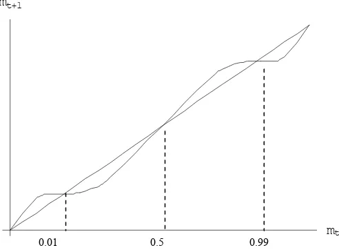
stage of consolidation. If we assign the values in Table 1 to the parameters, we have a situation as described above and shown in Figure 2.
In this case the system presents three internal equilibrium points,m∗
1≈0.01,
m∗
2 = 1−m∗1 ≈ 0.99 and m∗3 = 0.5 as well as two fixed points m∗4 = 0 and
m∗
5 = 1. In view of the perfect structural homogeneity of the tourist localities
and since|g′(m∗
1)|= 0.6734<1, the equilibriumsm∗1 andm∗2are locally stable.
Equilibrium m∗
3 is instead unstable, as |g′(m∗3)| = 1.44982>1. At time zero,
therefore, locality A is positioned at point mA,0 = m∗1 whilst, by symmetry,
locality B absorbs almost all the tourist flow available and positions itself at
1−mA,0=m∗2.
5 5 max 10 ˆ ˆ 10 2 1 10 100 parameters l Conditiona 01 . 0 5 . 0 parameters l conditiona -Non = = = = = = = = = = = = = = B A B A B A B A B A B A E E M c c N N β β α α σ ε ε
Table 1: base values for the numerical simulation of
the model.
Starting from the basic case with the parameter values shown in Table 1, one
of the parameters will be varied each time in conditions of ceteris paribus. In
order to assess the effect produced by economic policies, the parameters that can be conditioned by public intervention are kept distinct from those that cannot be directly influenced by policy measures.
mt mt+1
0.01 0.5 0.99
Figure 2: Initial state of the system. Locality A is in a stable equilibrium positionm≈0.01,
whilst locality B is in stable equilibrium m ≈ 0.99. The point of equilibrium m = 0.5 is unstable.
The following parameters belong to the first category:
a. Parameters α and β for environmental impact (of tourists and firms
[image:15.595.176.422.411.592.2]b. The number of firms working in the industry (Nd), which can be modified
by adopting appropriate industrial policies to favour or reduce competi-tion;
c. Costs (cd), which can be affected by subsidies for the production of tourist
services and incentives for the use of efficient technologies and tax conces-sions.
The second type includes the parametersσandǫdwhich describe the tastes
and price sensibility of tourists and therefore are beyond the direct control of
public authorities. The parameter σis an indicator of the criterion followed by
a tourist in his choice of the locality to be visited: an increase means greater sensibility to the real benefits obtained by visiting a certain locality rather than its reputation; its value will depend therefore on factors linked to lifestyle and
fashion. ǫd represents the perception that the tourist has of the service that
he is offered: the closer the value is to 1 (rigid demand), the more the service
is perceived as a luxury good; in the same way, a low value of ǫd implies high
elasticity of demand and therefore an increased sensibility to price associated
with mass tourism14.
In each of the simulations, the key element is the bifurcation diagram which, given a certain initial state, describes the long term behaviour of the system in relation to variations in a parameter. The chosen parameter is made to vary within a specific interval in 500 steps; the orbit is calculated for at least 400 periods for each value of the parameter considered in the specified interval. However, in order to highlight the long term behaviour, the diagram shows only the last 150 repetitions; that is, for each value of the parameter, the bifurcation
diagram representsg[t](m
A,0) for 250≤t≤τ withτ ≥400.
3.1
Changes in demand elasticity -
ǫ
Let us analyse the case in which, starting from a situation of equilibrium as described in Figure 2, a change in demand elasticity takes place for locality
A. Although the two localities under consideration are supposed to be
struc-turally identical, it is possible that at a later stage differences in their level of development change the tourist’s sensibility to price according to the locality visited. For example, given the negative effects of congestion and productive activities on the environment, the tourist may develop a greater sensibility to price with a consequent increase in demand elasticity for the destination with a larger number of visitors. On the other hand, the less developed locality is still able to offer a high level of environmental quality, thus encouraging the tourist to accept a higher price for the same service. The opposite situation may also occur, where the less developed locality ends up with a higher demand elasticity as the tourist is more sensitive to the reputation of a destination rather than
its quality. These considerations persuade us that variations in parameter ǫA
are possible in all directions. In general, a tightening of demand (increase in
ǫA ) leads to an improvement in the quality of the environment and a
conse-quent increase in the surplus ScA. It is more likely, therefore, that condition
14We assume that the two localities can present different levels of demand elasticity. This
eσ·ScA,0m
A,0 > eσ·ScB,0(1−mA,0) prevails with the tourist flow beginning to
move from B to A. On the other hand, an increase in elasticity can start an
inverse mechanism and lead to the decline of destination A, even before this
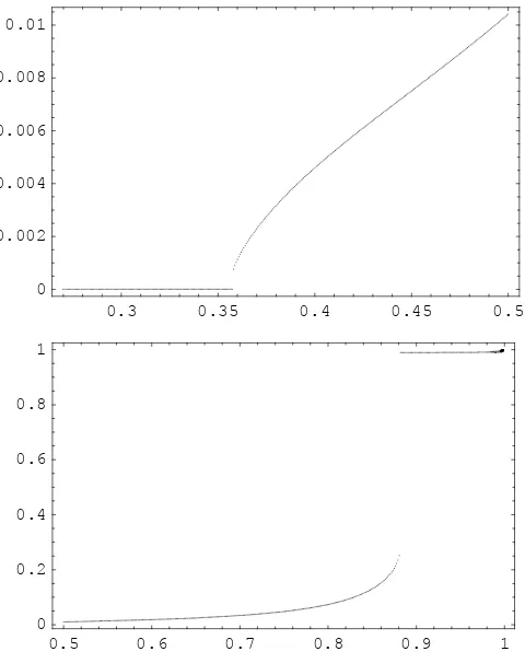
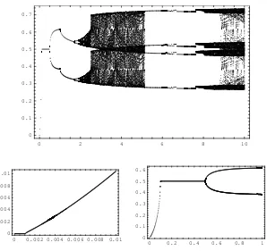
locality begins to attract a significant share of the tourists. Figure 3 shows the
bifurcation diagram where we indicate the interval of the values for ǫA with
I = (0,1) to facilitate the reading of the diagram, before subdividing it into
three subintervalsI={I1, I2, I3} to identify the different parts of the diagram
which show the behaviour of the system to be basically homogeneous:
1. ǫA∈I1= (0, ǫ1≈0.35): locality A experiences a gradual loss of visitors
to the competing locality. In the long term all the tourists settle inB;
2. ǫA∈I2= [ǫ1, ǫ2≈0.88): locality Amanages to keep a small share of the
potential tourists who continue to prefer alternative destinations;
3. ǫA ∈ I3 = [ǫ2,0.999): there is a radical change in the dynamics of the
development of destination A which, given the low elasticity of demand and the consequent increase in the surplus of a tourist, is now able to attract a substantial share of tourists.
0.3 0.35 0.4 0.45 0.5 0
0.002 0.004 0.006 0.008 0.01
0.5 0.6 0.7 0.8 0.9 1 0
[image:17.595.182.422.355.658.2]0.2 0.4 0.6 0.8 1
Figure 3: Bifurcation diagrams in relation toǫA with the initial statem0 ≈0.01. xaxis:
ǫA;yaxis: mA.
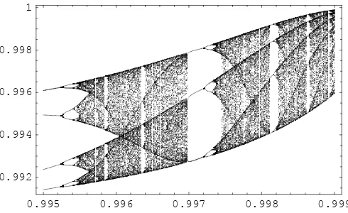
A first reading of the diagram therefore seems to suggest general stability
however, reveals elements of a more complex nature. Figure 4 shows two details of the bifurcation diagram in which the long term dynamics do not seem to converge to a fixed value, but instead become cyclical, confirmed by the presence of bifurcations, or chaotic. The existence of cycles of any order and chaotic trajectories is confirmed by the presence of a cycle in period 3 (Li-Yorke theorem,
1975)15, which is very evident in the central part of the detail on the right.
0.98 0.9825 0.985 0.9875 0.99 0.9925 0.995 0.9975 0.99
0.992 0.994 0.996 0.998 1
0.995 0.996 0.997 0.998 0.999 0.992
[image:18.595.176.421.409.559.2]0.994 0.996 0.998 1
Figure 4: Details of the bifurcation diagram shown in Figure 3. For the values ofǫA close
to 1 the dynamics in the long run take on chaotic or cyclical trends. xaxis: ǫA;yaxis:mA.
15On the basis of the Li-Yorke theorem (1975):
Given a continuous functionmt+1=g(mt)at intervalJ→J⊂ ℜand supposing that point
m∈Jexists such that
g[3](m)≤m < g(m)< g[2](m)
then
i for eachn= 1,2,3....there exists a trajectory of periodninJ;
Even if these observations are not particularly significant as they are located
in an interval with limited values16, they do, however, show an important
prop-erty of the model, namely, it generates endogenously complex dynamics in the development of a tourist locality. These complexities will become evident in later simulations. Another important aspect emerges when the trajectories of
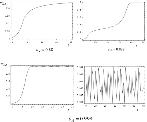
the tourist flow with specific values ofǫAare simulated. As the graphs in Figure
5 show, the dynamics of the tourist flow follow the type of trend theorised by Butler. The interesting point is the difference in the behaviour of the cycle in
the post-consolidation phase. In the first simulated case (ǫA = 0.88) the cycle
tends to become stable following the period of consolidation with a phase of stagnation; in other cases, growth picks up again with a new Butler-type cycle
(ǫA= 0.888) and an infinite series of chaotic oscillations begins (ǫA= 0.998).
On the basis of the values assigned to the parameters, the maximum
sustain-able tourist flow is positively correlated with the elasticity of demand 1/ǫd, that
is ∂mˆd/∂ǫd <0 and, given that in the case we analysed high values of ǫA are
combined with a significant growth in the tourist flow towards destinationA, it
is possible that, at those values, there emerges a condition in the industry that
was environmentally unsustainable, that ismA,t>mˆA. For example, in the case
analysed above in whichǫA= 0.998, the maximum limit of sustainable tourism
becomes ˆmA= 0.835, well below the values of the tourist flow which, even with
an irregular trend, is always more than 99% of the total tourist population, as seen in the details in Figure 5.
0 5 10 15 20 0
0.05 0.1 0.15 0.2
0 10 20 30 40 50 0
0.2 0.4 0.6 0.8 1
0 5 10 15 20 25 30 0
0.2 0.4 0.6 0.8 1
0 10 20 30 40 50 60 0.994
0.995 0.996 0.997 0.998 0.999 88
. 0
=
A
ε εA=0.888
998 . 0 =
A ε
t A
m,
t A
m,
t t
[image:19.595.167.424.403.617.2]t t
Figure 5: Time series of the tourist flow towards destination A with different values ofǫA.
In the first two cases the flow converges towards a stationary state and in the third towards a seemingly stable phase, but it is in fact characterised by chaotic irregularities. xaxis: t;y
axis: mA,t.
16Although it follows chaotic trajectories, the tourist flow is always close to 99.5% of the
Following the same reasoning, environmental unsustainability can be shown
in the case in whichǫA= 0.888 with ˆmA= 0.871 and sustainability forǫA= 0.88
with ˆmA = 0.873. In general, development appears sustainable so long as
ǫA < ǫ2 ≈0.88 whilst for higher values the number of visitors grows so much
that it exceeds the maximum sustainable limit.
3.2
Changes in the criterion for the choice of locality -
σ
Parameterσis an indicator of the criterion followed by the tourist in his choice of
locality17: if it increases, it means less attention is being paid to the reputation
of a certain tourist locality and more to the real benefit that can be obtained;
if σ is low, the tourists tend to stay in B, given that the rival locality is not
sufficiently attractive since it is still in the initial phases of development.
At time zero the system is in equilibrium, that iseσ·ScA,0m
A,0=eσ·ScB,0(1−
mA,0) withmA,0≈0.01041. This condition can be rewritten asσ·(ScA,0−ScB,0) =
ln1−mA,0
mA,0
with, given perfect structural homogeneity and as ∂Scd
∂md < 0 ∀d,
ScA,0> ScB,0 ifmA,0<0.5. Following variations inσ, therefore, the system is
going to be in disequilibrium with the result that there will be a flow of tourists
towards locality Aifσincreases and away from it if it decreases.
The bifurcation diagram in Figure 6 shows this trend and highlights the
increasing complexity of the dynamics asσincreases.
When the choice of a tourist destination is guided by fashion and evidence of
a greater number of visitors (low level ofσ), the tourist flow tends to be stable in
so far as it is difficult for the new tourist localities to attract tourists away from well-established destinations. If the choice is taken in a more rational way, that is, privileging those localities that guarantee a higher level of well-being, it is likely that the tourist flow will begin to move towards the less visited localities, before starting to fluctuate cyclically or chaotically from one locality to another, following the continuous oscillations in the levels of surplus that can be obtained in each one of them.
The simulation was limited to an interval with the valuesσ∈[0,10], without
substantial changes in the behaviour of the system for wider intervals.
The study of the dynamics in the long term is made, as above, by dividing the interval into three specific subintervals:
1. σ ∈ [0, σ1≈0.1): the flow of tourists tends to abandon locality A with
values ofσclose to zero and to reach a stationary level forσ→σ1≈0.1;
2. σ∈[σ1, σ2≈0.5): the tourist flow tends to settle equally at both tourist
destinations;
3. σ ∈ [σ2,10): the long term trajectories of the tourist flow have mostly
cyclical or chaotic behaviours, showing evident fluctuations in a wide in-terval that goes from 30% to 70% of the total tourist population.
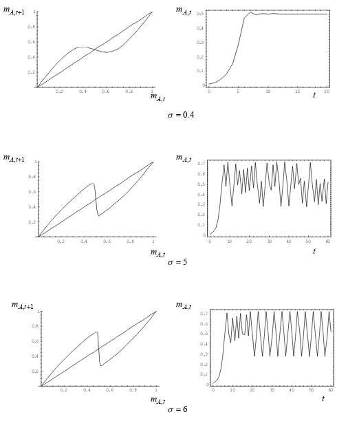
Figure 7 shows three possible developments of the tourist flow, which
corre-spond to the same number of values for parameterσ. Cycles, chaos and
asymp-totic convergence are possible future developments of a tourist destination, but
17Given the values in Table 1 and thatσdoes not directly condition tourists’ surplus, the
two localities remain structurally homogeneous, independently of the value of this parameter. The set of fixed points in the system therefore also includesm∗
0 2 4 6 8 10 0
0.1 0.2 0.3 0.4 0.5 0.6 0.7
0 0.002 0.004 0.006 0.008 0.01 0
0.002 0.004 0.006 0.008 0.01
0 0.2 0.4 0.6 0.8 1 0
[image:21.595.151.449.271.552.2]0.1 0.2 0.3 0.4 0.5 0.6
Figure 6: Bifurcation diagram with respect to parameterσwith an initial statemA,0≈0.01.
0.2 0.4 0.6 0.8 1 0.2 0.4 0.6 0.8 1
0 5 10 15 20
0 0.1 0.2 0.3 0.4 0.5
0.2 0.4 0.6 0.8 1
0.2 0.4 0.6 0.8 1
0 10 20 30 40 50 60
0 0.1 0.2 0.3 0.4 0.5 0.6 0.7
0.2 0.4 0.6 0.8 1
0.2 0.4 0.6 0.8 1
0 10 20 30 40 50 60
0 0.1 0.2 0.3 0.4 0.5 0.6 0.7 1
,t+ A m
1 ,t+ A m
[image:22.595.172.417.249.555.2]1 ,t+ A m t A m, t A m, t A m, t t t t A m, t A m, t A m, 4 . 0 = σ 5 = σ 6 = σ
Figure 7: Time series of the tourist flow and the corresponding Staircase Diagram for the
different values of σ. The tourist flow converges towards a stationary state in the first case and follows a chaotic and cyclical trend in the second and third cases respectively. xaxis: t;
the element which is common to each one of the scenarios is the Butler-type initial growth phase. In all three cases, the stagnant, chaotic or cyclical phase emerges only after a first phase of marked development that takes more than
50% of potential tourists to localityA.
With reference to the sustainability of the environment, variations inσ do
not change the maximum level of sustainable tourism, which therefore remains
constant. As ˆmA = 0.98 and observing how the share of tourist population
never exceeds 80%, we can conclude that the condition of sustainability is always
satisfied with each value ofσin the interval considered.
3.3
Changes in the number of firms (
N
) and marginal cost
(
c
)
Considering Ωd= Ncdd−Nǫdd we can rewrite the expression of surplus as
Scd=
ˆ
Ed−αMd+ 1
1 +βMdΩ1d/ǫd
· ǫd
1−ǫd
·Ω
1−ǫd
ǫd
d if Ed,t>0
Scd= 1−ǫdǫd·Ω
1−ǫd
ǫd
d if Ed,t ≤0.
Surplus and therefore the dynamic equation of the model depend on the
number of firmsNd∈ ℵand production costscd>0 by means of the factor Ωd;
we can then study the effect produced by variations in one or both parameters
through variations in that factor. IfEA,t>0 and for a given value of a tourist
Ωˆ *
A
Ω eq
A
Ω ΩA Ω
~
A Ω
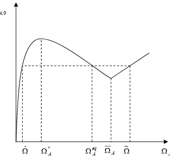
[image:23.595.216.385.454.613.2]0 , A Sc
Figure 8: Surplus function of the tourist who visits locality A at timet= 0. For ΩA<Ω¯A
the function takes on the form of a parabola with a maximum in Ω∗
A. If ΩA>Ω¯Athe function is linear and growing.
flowmA,t∈(0,1), surplus is first a growing function of ΩA, before falling once
the maximum point has been reached Ω∗
A =
1−ǫA ǫAβMA
ǫA
become too high, the locality can undergo a sudden reduction in size because of excessive environmental costs. Nevertheless, there is also a second effect on surplus, this time connected with variations to the maximum limit of sustainable
tourism ˆmAcaused by ΩA. This limit tends to decrease as ΩAgrows, thus there
will be a ¯ΩAsuch that the maximum limit of sustainable tourism is lower than
the actual level of tourism, ˆmA < mA,t, for all ΩA > Ω¯A so that the tourist
industry is no longer sustainable in terms of the environment (Ed,t= 0), and
surplus becomes a growing monotone function of ΩA.
Given the initial equilibrium condition (mA,0≈0.01041) and the values
as-signed to the parameters, we obtain ˆΩ ≈ 0.0048, Ω∗
A ≈ 0.0219, ¯ΩA ≈ 6.89,
˜
Ω ≈ 455.5 and ΩeqA = 0.0995 where ΩeqA indicates the value of the parameter
in the initial equilibrium state. The situation before the variation in ΩA is
de-scribed in Figure 8 and on that basis we could expect, in relation to the starting
point, a fall in the tourist flow for ΩA <Ω and Ωˆ eqA <ΩA <Ω, an increase for˜
ˆ
Ω < ΩA < ΩeqA and ΩA > Ω, with˜ ScA
ˆ
Ω =ScA(ΩeqA) = ScA
˜
Ω, as the
bifurcation diagrams confirm in Figure 9.
0 0.01 0.02 0.03 0.04 0.05 0.06 0
0.2 0.4 0.6 0.8 1
460 480 500 520 540 560 580 600 0
0.2 0.4 0.6 0.8 1
500 520 540 560 580 600
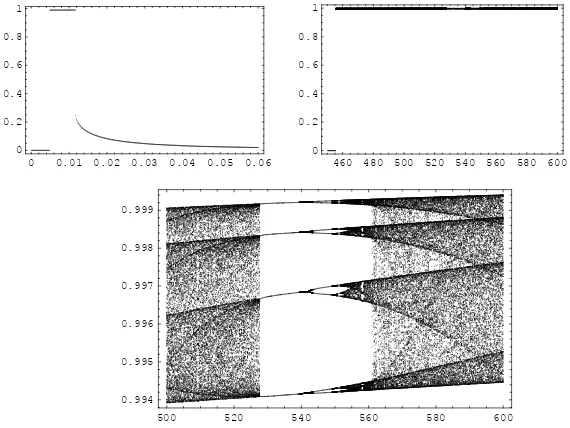
[image:24.595.159.444.337.551.2]0.994 0.995 0.996 0.997 0.998 0.999
Figure 9: Bifurcation diagram with respect to ΩA in the initial conditionmA,0≈0.01. x
axis: ΩA;yaxis: mA.
Peaks of tourist flows can be observed for ΩA∈(Ω1≈0.005) , Ω2≈0.01173
and ΩA > Ω3 ≈455.53. In this last case, however, the detail in the diagram
for interval 500 < ΩA < 600 , shows how the final phase of development in
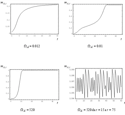
the tourist industry presents unstable or cyclical trends, even if they are on the whole insignificant, because they are within a very small interval of values given that the tourist flow is always higher than 99% of the total population of tourists. In Figure 10 three possible paths of development are shown for locality
A. In the first case, ΩA= 0.012, development follows the typical phases of the
Butler cycle before stabilizing around 20% of the total tourist population; in the
second case, ΩA= 0.01, growth follows a double Butler-type cycle that remains
consists in a single Butler cycle culminating in an apparently stable phase, but in fact, it is marked by continuous chaotic fluctuations, as shown for the 60
periods that go fromt= 15 tot= 75.
The results of the simulation lead to some important considerations. The
fact that development can be made by either increasing or reducing ΩA leaves
industrial policy ample room for manoeuvre. The two types of intervention, however, present substantial differences both in terms of practicability and en-vironmental sustainability. If tourist development is to be started by increasing
ΩA, the measures will have to be such that ΩA>Ω3, which requires a
substan-tial increase in the number of firms together with a significant reduction in the costs of production, but this is not always practicable.
On the other hand, decreases in ΩAcan generate development, but only for
values included in a limited interval. If the reduction is excessive, the industry will lose all chance of growth, whereas development will have a limited effect on small shares of the tourist population if the decrease is not sufficiently strong. As a consequence, policy errors can compromise the future development of tourist destinations or at least reduce its impact.
The first type of intervention therefore seems preferable, since it allows both
the full development of the locality, even where ΩAincreases excessively, and a
reduction in the level of prices, as p∗
d = 1/Ωd. This reasoning, however, does
not give enough attention to the environmental implications of the two different
industrial policies. Increases in ΩA, in fact, reduce the maximum limit of
sus-tainable tourism, thus making this policy unadvisable from an environmental
point of view. More specifically, as ˆmA ≈0 ∀ΩA>Ω3, no value of ΩA higher
than Ω3 is capable of guaranteeing sustainable development, which would be
possible if ΩA were reduced, so that we obtained ΩA ∈ (Ω1,Ω2) given that in
this case we would have ˆmA≈1.
0 5 10 15 20 25 30 0
0.05 0.1 0.15 0.2
0 10 20 30 40 0 0.2 0.4 0.6 0.8 1
0 10 20 30 40 0 0.2 0.4 0.6 0.8 1
0 10 20 30 40 50 60 0.994 0.995 0.996 0.997 0.998 0.999 t A
m, mA,t
t A
m, mA,t
012 . 0
=
ΩA ΩA=0.01
520 = ΩA t t t t 75 a 15 da
520 = =
=
[image:25.595.196.397.463.648.2]ΩA t t
Figure 10: Time series of tourist flows in A for different values of ΩA.
The fact that the state of chaos (or cyclicity) in the long term occurs with
very high values of ΩA but does not bring about significant fluctuations to
parameters. Therefore, a very different picture emerges if, for example, the
simulation is repeated hypothesizing that at time zero parameterσmoves from
0.01 to 1.
0 0.0001 0.0002 0.0003 0.0004 0.0005 0
0.2 0.4 0.6 0.8
0 5 10 15 20 25
[image:26.595.187.410.174.495.2]0 0.2 0.4 0.6 0.8
Figure 11: Bifurcation diagrams for ΩA withσ = 1 and an initial statemA,0 ≈0.01. x
axis: ΩA;yaxis: mA.
As Figure 6 shows, this structural variation would start a flow of tourists
away fromBtoA, until the flow stabilized in a cycle in period 218. Faced with
the prospect of growth, local institutions could decide to adopt expansionary policies to attract a greater number of firms and to reduce the price of tourist services or, at the same time, make the entry of new firms conditional upon specific investments capable of guaranteeing a high standard of services, with a consequent increase in the marginal costs of production and the equilibrium
price. Given that ∂ΩA/∂NA > 0 and ∂ΩA/∂cA < 0, the final effect of this
manoeuvre cannot be unequivocally determined, as it could lead to either an
increase in ΩA if the positive effect of the proliferation of firms prevailed, or a
reduction, if the negative impact of production costs prevailed.
It is evident from the bifurcation diagrams in Figure 11 that the chaotic
nature of the paths of development emerges for both low and higher values of ΩA.
Furthermore, unlike the preceding case, the chaotic (or cyclical) fluctuations
are much bigger, which indicates that there can be important variations in the number of visitors from one period to another.
0.2 0.4 0.6 0.8 1
0.2 0.4 0.6 0.8 1
0 10 20 30 40 50 60 70
0 0.2 0.4 0.6 0.8 0004 . 0 = ΩA
0.2 0.4 0.6 0.8 1
0.2 0.4 0.6 0.8 1
0 5 10 15 20 25 30
0 0.1 0.2 0.3 0.4 5 . 4 = ΩA
0.2 0.4 0.6 0.8 1
0.2 0.4 0.6 0.8 1
0 5 10 15 20 25 30 35
0 0.2 0.4 0.6 0.8 5 . 14 = ΩA 1
,t+ A
m
1 ,t+ A
m
[image:27.595.199.400.163.461.2]1 ,t+ A m t A m, t A m, t A m, t A m, t A m, t A m, t t t
Figure 12: Time series of the tourist flow to A for different values of ΩA. The Staircase
Diagram is linked to each one of the time series that it generated starting from the initial statemA,0, withσ= 1.
Figure 12 shows three possible trajectories for development corresponding to
the same number of values of ΩA. As in the cases analysed above, the first phases
of development follow the typical trend of the Butler cycle, whilst the main differences can be seen in the post-consolidation phase; in the first and third case the dynamics become irregular and are probably chaotic, whereas in the second they converge towards a stationary state. As far as environmental sustainability is concerned, what was said above is true, as there are no variations in the limit
ˆ
mA following a change in σ. As∂mˆA/∂ΩA<0, development tends to absorb
growing quotas of environmental resources the higher the value of ΩA. To be
more specific, environmental sustainability is present only in the first of the three cases analysed in Figure 12 where the trajectories of the tourist flow, though showing obvious fluctuations, remain lower than the maximum sustainable limit
that is ˆmA ≈ 1 whereas in the other two cases the limit is exceeded by the
arrival of a larger tourist flow. To be more precise, for ΩA = 4.5 the locality
attracts about 50% of the tourist population when the maximum sustainable
limit is ˆmA≈0.024, whilst for ΩA= 14.5 the flow fluctuates chaotically between
environmental sustainability equal to ˆmA≈0.0023.
3.4
Changes in the environmental impact of tourists
(
α
)
and firms
(
β
)
The other parameters sensitive to economic policy measures concern the
conse-quences of economic activities (β) and the tourist flow (α) on the environment.
We will limit the analysis to the study of the effects produced by variations in
the parameters of environmental impact on localityA, first with two simulations
for the variations inαA and βA, respectively, then with a third where the two
parameters are made to vary together. Certainly these three simulations do not exhaust all the possible cases, but we believe that they are sufficient to test whether, starting from a condition of stability in the long term, the economic policies that change the environmental impact of productive activities and the
tourist flow have the capacity to destabilise the system19.
Changes in αA: the system is stable for the whole interval of values
consid-ered,αA∈(0,10). Reductions in the environmental impact of the tourist flow
are not sufficient to guarantee the beginning of significant development in the tourist locality, which continues to attract little more than 1% of the potential
tourist population forα <1 (figure 13).
0 2 4 6 8 10
[image:28.595.164.436.381.542.2]0.0094 0.0096 0.0098 0.01 0.0102 0.0104
Figure 13: Bifurcation diagram forαA with initial statemA,0 ≈0.01. xaxis: αA;y axis:
mA.
We can define this situation as alock-in, as the system is in fact blocked in
its initial position, even after a significant change in the environmental impact of the tourist flow (Faulkner-Russel, 1997).
However, it is sufficient that, as in the previous simulation, an increase from
0.01 to 1 in parameterσoccurs at time zero for the behaviour of the system to
change radically.
The diagrams in Figure 14 show a marked complexity in the dynamics of the tourist flow in this case. The popularity of a tourist destination plays a less
19Alternative scenarios could emerge if policy measures affecting the parameters of
environ-mental impact involving both tourist destinations were considered; in this caseαA=αBand
important role in the choice of tourists and localityAcan therefore hope for a greater flow of visitors.
0 0.5 1 1.5 2
0.3 0.4 0.5 0.6 0.7
0 2 4 6 8 10
[image:29.595.204.396.161.437.2]0.1 0.2 0.3 0.4 0.5 0.6 0.7
Figure 14: Bifurcation diagram forαAwith initialmA,0≈0.01 andσ= 1. xaxis: αA;y
axis: mA.
Development is all the greater, the lower the value ofαA . However, if the
interval of values between α1 ≈ 0.5 and α2 ≈ 1.5, in which the trajectories
are periodic in period 2, is omitted, the tourist flow appears generally complex with big cyclical or chaotic fluctuations. This complexity is not present in the
previous case with σ = 0.01. Figure 15 shows two possible developments for
αA= 0.05 and αA= 4; once again, what seems to be the first phase of
Butler-type development is followed by an indefinite series of apparently chaotic
fluc-tuations20.
If the environmental impact of tourist flows is reduced, the maximum level of sustainable tourism can be increased. It can be immediately verified that, for
αA ≤α¯ ≈0.98, ˆmd ≥1 is obtained, so that, whatever the level of the tourist
flow in a certain period, locality A will be able to grow without compromising all its natural resources. On the other hand, growth is also possible for higher
values of αA, which are higher than they were at the beginning, although in
this case growth is more contained and there is a risk of using all the available
environmental resources. For αA= 4, for example, the maximum level of
sus-20Enlargements of the diagram in figure 14 (not shown in the text) reveal the presence of
tainable tourism becomes ˆmd≈0.248 which, as shown in figure 15, is frequently
exceeded by much higher levels of tourists arriving.
0 10 20 30 40 50
0 0.2 0.4 0.6
0 10 20 30 40 50 0
0.05 0.1 0.15 0.2 0.25 0.3 t
A
m, mA,t
t t
05 . 0 = A
[image:30.595.149.445.170.291.2]α αA=4
Figure 15: Time series of the tourist flow to A for different values ofαA,σ= 1.
Changes inβA: even in the presence of a strong ’popularity effect’ generated
by a low value ofσ, Figure 16 shows how the reductions ofβAare, at least in this
case, more effective in favouring development in the tourist industry. It is, in fact, possible to attract a larger share of visitors by reducing the environmental impact of firms, even after starting with a small number of visitors, but in a context in which reputation plays a central role in attracting them.
0 0.5 1 1.5 2
0 0.1 0.2 0.3 0.4 0.5 0.6 0.7
Figure 16: Bifurcation diagram forβA with initial condition mA,0 ≈0.01. xaxis: βA;y
axis: mA.
The details of the diagram shown in Figure 17 reveal that the trajectories
of the tourist flow tend towards a stationary state for ¯β≈0.038≤βA≤2 and
to follow a cyclical or chaotic trend for 0≤βA≤β¯.
An example is given in Figure 18 forβA= 0.001; in this case the first phase,
[image:30.595.163.439.412.585.2]0 0.01 0.02 0.03 0.04 0.3
0.4 0.5 0.6 0.7
0.05 0.1 0.15 0.2 0.25 0.3 0.35 0.4
[image:31.595.203.398.266.551.2]0.1 0.2 0.3 0.4 0.5 0.6
impact. Figure 18 also shows the path of development for βA = 0.16; the flow
can be seen to become stationary around 50% of the total tourist population. The differences between the previous case and this one, however, are not to be found just in the different behaviour of the flow in the post-consolidation phase, but also, and above all, in the time necessary to complete that phase. In the
first case, with a very lowβA, 70% of the tourist population can be reached in
just 7 periods, after which the flow begins to fluctuate irregularly, whilst in the second case growth is gradual, requiring more than 30 periods to reach half the potential tourism.
0.2 0.4 0.6 0.8 1 0.2
0.4 0.6 0.8 1
0 10 20 30 40 50 60 0 0.1 0.2 0.3 0.4 0.5 0.6 0.7 001 . 0 = A β
0.2 0.4 0.6 0.8 1 0.2
0.4 0.6 0.8 1
0 5 10 15 20 25 30 35 0 0.1 0.2 0.3 0.4 0.5 16 . 0 = A β 1 ,t+ A m
[image:32.595.156.445.253.504.2]1 ,t+ A m t A m , t A m , t A m , t A m , t t
Figure 18: Time series of the tourist flow to A for different values ofβA.
The development is sustainable in environmental terms, as it is for all values
ofβAbelow 2, as ∂mˆA/∂βA<0 and ˆmA≈0.98 forβA= 2.
Changes inαA, βA: as the analysis allows the study of only one parameter at
a time through the bifurcation diagram, we can hypothesiseαA/βA will always
be constant and αA = (1 +h), βA = 2 (1 +h) with h∈[−1,∞). In this way
we can study the effect of variations in the two parameters of environmental
impact simply by observing what happens by varying parameterh.
The parameters of environmental impact are reduced withh < 0. In this
case, although the lower values of pollution substantially increase the number
of visitors to localityA (figura 19), the development that will start can follow
very different trends, depending on the size of the reduction. Figure 20 shows
different sections of the bifurcation diagram for h <0. In the first interval of
values, h∈ (h1≈ −0.978,0], the system remains stable, with trajectories
con-verging towards a stationary state. Further reductions, withh∈(h2≈ −1, h1],