Evolving extended naive Bayes classifiers

Evolving Extended Na¨ıve Bayes Classifiers

Frank Klawonn

Department of Computer Science

University of Applied Sciences BS/WF

Salzdahlumer Str. 46/48

D-38302 Wolfenbuettel, Germany

f.klawonn@fh-wolfenbuettel.de

Plamen Angelov

Department of Communication Systems

InfoLab21

Lancaster University

South Drive, Lancaster LA1 4WA, UK

p.angelov@lancaster.ac.uk

Abstract

Na¨ıve Bayes classifiers are a very simple tool for classi-fication problems, although they are based on independence assumptions that do not hold in most cases. Extended na¨ıve Bayes classifiers also rely on independence assumption, but break them down to artificial subclasses, in this way becom-ing more powerful than ordinary na¨ıve Bayes classifiers. Since the involved computations for Bayes classifier are ba-sically generalised mean value calculations, they easily ren-der themselves to incremental and online learning. How-ever, for the extended na¨ıve Bayes classifiers it is necessary, to choose and construct the subclasses, a problem whose answer is not obvious, especially in for online learning. In this paper we propose an evolving extended na¨ıve Bayes classifiers that can learn and evolve in an online manner.

1. Introduction

In recent years, in many application fields of data anal-ysis and mining it was realised that there is a strong need for analysing and mining streaming data. Streaming data differ from the classical paradigm of data analysis and min-ing in the sense that the data set to be analysed is not com-pletely available at the start of the analysis. Data arrive as a stream so that more and more data become available over time. In most applications it is not possible to wait until a large amount of data has been collected for the analysis. Instead, the analysis should be started as soon as possible, even with a small data set. However, when more data arrive, the analysis should not be re-started completely, but should be carried out in an incremental fashion. This means that new or modified algorithms are needed that can work in an incremental way. In most cases, it is also impossible to store the full history of the data stream. Therefore, an algorithm for streaming data should only rely on a small, simplified

excerpt from the original data stream that contains the nec-essary information for the analysis.

When a data stream is analysed in a purely incremen-tal fashion, it is assumed that the underlying model of the data and its parameters do not change over time, which turns out to be an unrealistic assumption in many applica-tions. Therefore, a proper analysis of a data stream must be able to evolve over time, i.e. it must be able to adjust its model structure and the corresponding parameter set, when changes in the data stream occur.

In this paper we focus on evolving classifiers. This means we assume that the data stream consists of a num-ber of input attributes that are used for the prediction of an additional categorical attribute whose values are the classes. The correct classification is not available at the time, when the input data arrive and the prediction is needed. How-ever, in order to be able to train the evolving classifier, we assume that the correct classification will be available at a later stage. For instance, when we want to predict whether it will rain the next day, the prediction must be based on known measurements available before the next day. How-ever, after the next day, it is known whether the prediction was correct or not, i.e. whether it has been raining or not.

in order to achieve a better performance. Another advan-tage of extended na¨ıve Bayes classifiers is that they can be interpreted as a rule-based fuzzy classifier so that their clas-sification behaviour is easier to understand for non-experts. The evolving extended na¨ıve Bayes classifier proposed in this paper can handle continuous as well as categorical attributes. Updating the parameters of the probability dis-tribution can be carried out in a purely incremental fashion, but it is also possible to neglect the influence of classifica-tions that were learned a long time. The more interesting evolving part of the classifier is the introduction of new ar-tificial subclasses in order to improve the performance of the classifier.

Section 2 briefly reviews the concepts of standard and extended na¨ıve Bayes classifiers and their relation to fuzzy classifiers. How incremental learning and evolving strate-gies can be applied to extended na¨ıve Bayes classifiers is discussed in section 3, followed by a brief example in sec-tion 4. We conclude the paper by outlining future work, especially ideas for simplifying the extended na¨ıve Bayes classifiers in an evolving fashion.

2. The Framework of Extended Na¨ıve Bayes

Classifiers

Supervised classification refers to the problem to predict the value of a categorical attribute, the so-called class, based on the values of other attributes that can be categorical, or-dinal or continuous. A typical setting for supervised classi-fication is where a data set of classified data objects is avail-able and the task is to construct the classifier based on this data set. Usually the data set is split up into a training and a test set, even multiple times in the case of cross-validation, in order to better judge the prediction quality of the classi-fier for unknown data. Typically, the misclassification rate is used as an indicator for the quality of the classifier. How-ever, this is only a special case of a general cost or loss ma-trix that specifies the estimated average costs that will result from misclassifications of an object from each true class to any other class . The misclassification rate simply uses a cost matrix with ones everywhere, except in the diago-nal. The costs in the diagonal, i.e. the losses for correct classifications are assumed to be zero. The costs for mis-classifications can differ extremely so that simply counting the misclassifications might mislead the classifier. If, for in-stance, we want to predict whether a component of a safety critical system like an aeroplane will work without failure during the next operation, the costs for misclassifying the component as faulty, although it would work, are the costs for exchanging the component. The costs for misclassifying a faulty component as correct can cause the death of many people as ”costs”.

A large variety of classifiers exist in the literature which

cannot be mentioned here completely. Linear discriminant analysis is a very simple statistical classifier that is easy to construct. Decision trees are very popular because they are easy to understand according to their simple rule-like struc-ture. The same applies to fuzzy classifiers. Both of them rely on more complex learning algorithms. Na¨ıve Bayes classifiers, that will be the focus of this paper, are also very elementary probabilistic models. They are Bayesian net-works with an extremely simple structure. The learning al-gorithm for na¨ıve Bayes classifiers is very simple and they can also be interpreted easily due to the – sometimes unre-alistic – underlying independence assumptions.

2.1. Na¨ıve Bayes Classifiers

A Bayes classifiers exploits the Bayes rule from

statis-tics:

(1)

is the hypothesis, in the case of classification any value of the categorical attribute that we want to predict. is the evidence, i.e. the information from the observed attributes that we want to exploit to predict the considered categorical attribute. When the misclassification rate is used as an indi-cator for the quality of the classifier, then simply the class

yielding the highest posterior probability

is predicted. If a cost matrix for misclassifications is known, the prediction tries to minimize the expected loss. If the categorical attribute to be predicted can take values from the finite set of classes , then the entry

for any

in the cost matrix stands for the costs that will result, when predicting

instead of the correct class . Of course, we always assume

!

for any"

. Cor-rect predictions do not cause any loss. The expected loss given evidence and predicting class

is

loss

# $

%'&)(+*

$

%&(+*

-,

(2)

In this case, the class

yielding the lowest value in (2) is predicted by the Bayes classifier.

Note that in both equations (1) and (2), the probability of the specific evidence does not have any influence on the predicted class

, since can be considered as a constant factor independent of

. Therefore, for the decision in (1), it is sufficient to consider the likelihoods (unnormal-ized probabilities).

/

(3)

and in (4) we only need the relative expected losses

rloss

0 $

%'&)(+*

.

%&(+*

(4)

The evidence represents the measured or given val-ues of the attributes that we exploit for the prediction of the considered categorical attribute. For a na¨ıve Bayes clas-sifier (see for instance [15]) it is assumed that these at-tributes are independent given the classes. This means that, if

,,,

are the attributes used for prediction, we have

,,,

,,,+

(5)

In order to apply a na¨ıve Bayes classifier, the probabilities in (5) must be known. In case that the attributes

,,,

are categorical attributes, these probabilities can be esti-mated based on the corresponding relative frequencies in the available training data set.

For a continuous attribute

, it is necessary to estimate its (conditional) probability density function (pdf) % from the training data set. Once we have an estimation for the pdf %, the corresponding value %

is used in (5) instead of the probability

. This means the computed value

,,,

is no longer a probability, but a likelihood, i.e. an unnormalized probabil-ity.

In order to estimate the pdf %, it is usually assumed that % belongs to a class of parametric distributions, so that only the corresponding parameters of the pdf have to be estimated. A very typical assumption is that

is nor-mally distributed with unknown mean

% and unknown variance

% . Such parameters can be estimated from the training data set using the corresponding well-known for-mulae from statistics.

2.2. Extended Na¨ıve Bayes Classifiers

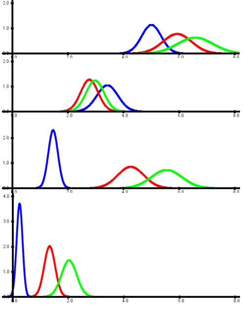
The underlying model of a na¨ıve Bayes classifier as-sumes that each class is characterised by a probability dis-tribution and for each class this probability disdis-tribution is simply the product of it marginals. Figure 1 shows the nor-mal distributions for the well known iris data set [3] learned by a na¨ıve Bayes classifier. The categorical attribute to be predicted has three different values for the iris data set. Four continuous attributes are used for the prediction. For each of the three classes, the na¨ıve Bayes classifier computes a four-dimensional normal distribution (with diagonal covari-ance matrices), whose marginal distributions are shown in figure 1.

The classification performance will work out well in cases like the iris data set, when the distribution of the data can be described roughly by a (multinomial) normal distri-bution for each class. If, however, the data objects of one

Figure 1. The normal distributions for the three classes for each of the four attributes for the iris data set.

class do not form a kind of compact cluster, but are dis-tributed over different separated clusters, then a na¨ıve Bayes classifier might fail completely.

In this sense a na¨ıve Bayes classifier can be viewed as a specific form of a fuzzy classifier using exactly one rule per class [10]. For this purpose the probability distribu-tions must be scaled in such a way that they never yield values greater than one, in order to interpret them as fuzzy sets. This leads to a constant scaling factor that does not influence the classification decision. The fuzzy sets (scaled distributions) for one class are aggregated by the product operator. Typically, fuzzy classifiers use the minimum for this operation. However, the minimum often leads to se-vere restrictions [14] and the product is a possible alterna-tive. The prior probabilities for the classes correspond to rule weights.

allowed for each class. In terms of a Bayes classifier, each class is represented by a number of artificial subclasses. In order to classify a data object, such an extended na¨ıve Bayes classifier will first compute the posterior probabili-ties (likelihoods) for each pseudo-class in the same way as a standard na¨ıve Bayes classifier. The posterior probabili-ties (likelihoods) for the actual classes are simply obtained as the sums of the posterior probabilities (likelihoods) of the corresponding pseudo-classes.

Although the classification of new data object is obvi-ous for an extended na¨ıve Bayes classifier, it is not clear at all, how to estimate the prior probabilities and the cor-responding probability distributions for the pseudo-classes. The problem during the training phase or construction of the extended na¨ıve Bayes classifier is to decide to which of its subclasses an object of a specific class should be assigned. The problem will be treated in the following section.

3. Incremental Learning and Evolving

Ex-tended Na¨ıve Bayes Classifiers

Online learning from data streams should neither involve storing all historic data nor re-initiating the learning proce-dure from scratch, when new data objects arrive. Learn-ing strategies that rely directly on the information given by wrong and correct classifications of the single data objects are usually not well-suited for online learning and need spe-cial adaptations. A typical example for classifiers working on this basis are most of the fuzzy classifiers [9]. Learning in decision trees is mainly based on a suitable impurity mea-sure like entropy. Since entropy is based on discrete bility distributions in the case of decision trees, these proba-bility distributions can be updated in an incremental fashion and corresponding approaches to online learning for deci-sion trees can be derived [6, 7]. However, this idea causes problems, when continuous attributes are considered for a decision tree and the splitting/discretisation of the contin-uous attributes should be carried out in an online fashion without storing all the data. For probabilistic models, when they use some general weighted mean concept to estimate their parameters, online learning is very easy to be imple-mented, as we will see in the following.

3.1. Advantages of Weighted Mean Concepts

A mean value

can be updated easily in an incremental manner by

, (6)

To update a mean value, it is sufficient to know the mean value of the previous observations, the new observation and

the number of observations. Note that the concept of a mean value, respectively its estimation, is much more general. It applies also to derived concepts, especially to statistical mo-ments. This fact can be exploited to compute variances and covariances in an online fashion. For the empirical variance, we have $ , (7)

This means, the variance only involves the computation of the two means

and

, i.e. the first and second mo-ment.

The general idea of the Bayesian approach in statis-tics is to update probabilities based on new observations. Therefore, it is no wonder that there exist many incremen-tal learning approaches in the spirit of the general Bayesian idea [1, 5]. These concepts are applied to many statisti-cal methods like linear discriminant analysis [11], but also to Bayesian networks [4], classifiers [13] and especially to na¨ıve Bayes classifiers [12].

So far, we have only focused on incremental learning. Evolving systems do not only learn in an online fashion, but also adapt and change their structure while new data arrive. It is also important to notice changes in the data stream. A simple incremental strategy as (6) will slow down the learn-ing process with an increaslearn-ing number of data. The under-lying assumption in (6) is that all data objects contribute the same information to the actual system or classifier, no matter how old these data objects are.

(6) is nothing else than a specific convex combination of the previous mean

and the new observation

. One can also think of other convex combinations, for instance

(8)

with a fixed constant

. This corresponds to the well known idea of exponential decay of the information. After new observations the contribution of an observation to the mean will decrease in an exponential fashion to

. In terms of the Bayesian idea, this means that the probability for a new observation equal or similar to the last one is

, whereas the probability for an observation equal or similar to one that lies steps back is

.

One can also realise a sliding window concept of size for the mean easily, if it is possible to store a fixed number of

3.2. Incremental Learning for Extended Na¨ıve

Bayes Classifiers

The above mentioned concepts can be applied to a na¨ıve Bayes classifier in a straight forward manner. The prior probabilities

for the classes are nothing else than mean values for counting variables, so that (6) can be used. The same applies to the conditional probabilities

for discrete attributes

.

For continuous attributes it is necessary to assume a cer-tain type of distribution. When the distribution is deter-mined by a finite number of its moments, then again (6) is applicable. For instance, in the case of normal distribu-tions, we can estimate the first and second moment (as spe-cific mean values) in an incremental fashion and compute the variance from (7). It should be noted that it is not nec-essary to consider complicated distributions, for instance Gaussian mixtures. The reason is that we use an extended na¨ıve Bayes classifier and a Gaussian mixture could be rep-resented by usual normal distributions for a corresponding number of pseudo-classes.

When the incremental update is carried out according to (6), incremental learning will yield the same result as batch learning. Of course, we can also apply the ”exponential for-getting” (8) or a sliding window concept that are not equiv-alent to batch learning, since they treat the data in an asym-metric way.

There is one open question for the extended na¨ıve Bayes classifier that we have not answered so far. It is not clear which class to choose for updating the corresponding prob-ability distributions. For a standard na¨ıve Bayes classifier, the probability distributions for the class of the new ob-served object are updated. But since in an extended na¨ıve Bayes classifier one class might be represented by a number of classes, we have to choose one of the pseudo-classes. In case, the extended na¨ıve Bayes classifier has predicted the correct class for the new observed object, we update the probability distributions of the corresponding pseudo-class that had yielded the highest likelihood. We could also choose this pseudo-class in case of a misclassi-fication. Note that in this case, we would not choose the class with the highest likelihood from all pseudo-classes, but only from those that represent the correct class. However, we slightly deviate from this concept in case of misclassification. The reason is the way we construct the pseudo-classes in an online fashion as described in the fol-lowing.

3.3. Evolving Extended Na¨ıve Bayes Classifiers

So far, we have only described incremental learning but no adaptation that is expected from an evolving system. We initialise the extended na¨ıve Bayes classifier as a standard

na¨ıve Bayes classifier, i.e. we start with one pseudo-class per class. New pseudo-classes are introduced, when the misclassification rate or the average loss is too high. Since the misclassification rate and the average loss per class are also weighted mean concepts, they can be tracked in an on-line fashion as well.

When then misclassification rate or the average loss is too high and we decide to introduce a new pseudo-class, we assign the pseudo-class to the class for which we have the highest misclassification rate or the highest average loss, re-spectively. We also have to specify initial probability distri-butions for the attributes for the new pseudo-class and also the prior probability for the new pseudo-class.

For the introduction of new pseudo-classes, we apply the following strategy. When we create the initial na¨ıve Bayes classifier, we already introduce for each class a second hid-den pseudo-class. These pseudo-classes are not used for prediction. But we update the probability distributions for a hidden pseudo-class each time a misclassification occurred for an object of the associated class. In this way, the hid-den pseudo-classes can already start to adapt their proba-bility distributions to those objects that are misclassified, although they do not participate in the classification pro-cess. When a hidden pseudo-class is added to the actual pseudo-classes, because of an unacceptable high misclassi-fication rate or average loss for the associated class, we sim-ply use the probability distributions for the attributes that were computed for the hidden class. The prior probability for the new pseudo-class is calculated as follows. Note that we cannot simply use the tracked prior probability of the hidden pseudo-class, since otherwise the sum of the prior probabilities of all classes would exceed one. The prior probability of the associated class is the sum of all prior probabilities of the corresponding pseudo-classes. Now we include the corresponding hidden class, without increasing the prior probability of the associated class. Assume that the pseudo-classes associated with the corresponding class have prior probabilities

,,,

and that the prior prob-ability for the hidden pseudo-class was calculated as

. This means that the prior probability of the associated class is

. We define the new prior probabilities for the pseudo-classes by

(new)

,,,

where

,

standard parameters (uniform distributions for categorical attributes, standard normal distributions for continuous at-tributes. The prior probability is set to zero.

As mentioned above, when a new data object is classi-fied correctly, we update the probability distributions of the pseudo-classes of the extended na¨ıve Bayes classifier yield-ing the highest likelihood. When the new object is classi-fied incorrectly by the extended na¨ıve Bayes classifier, we update the probability distributions of that pseudo-class as-sociated with the correct class that was last added to the extended na¨ıve Bayes classifier.

When we have moved a hidden pseudo-class to the ex-tended na¨ıve Bayes classifier, we do not immediately move another hidden pseudo-class to the extended na¨ıve Bayes classifier after the next observation, since in most cases the misclassification rate or average loss will not drop imme-diately after introducing a hidden pseudo-class to the ex-tended na¨ıve Bayes classifier. Before we move another hid-den pseudo-class to the extended na¨ıve Bayes classifier, we wait a fixed number of new observations in order to give the modified classifier a chance to adapt its parameters.

4. An Application Example

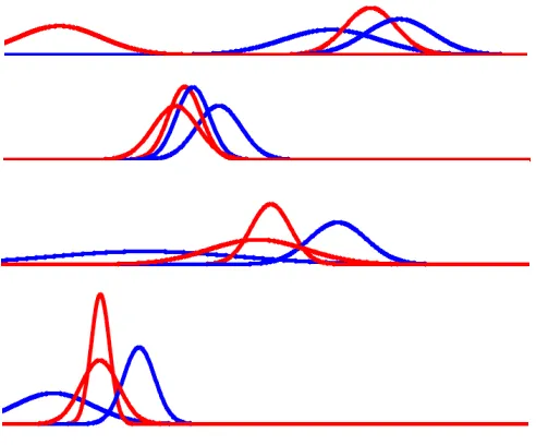
In order to illustrate how our approach works, we con-sider a modified version of the iris data set. The original iris data set contains three classes that are roughly grouped into three clusters. We artificially join two of the classes, so that one class is represented by two clusters. We then apply our incremental evolving extended na¨ıve Bayes classifier to a stream of randomly drawn samples from the iris data set. The classifier constructs four pseudo-classes, two for each class, i.e. one more than expected. Figure 2 shows the cor-responding normal distributions. Although the distributions do not completely look like one would expect, the misclas-sification rate is quite low (4%). The left normal distribution for the first attribute and the corresponding pseudo-class is almost not used by the classifier.

5. Conclusions

In this paper, we have proposed an extended version of a na¨ıve Bayes classifier that is able to learn in an incremental fashion and to extend its structure automatically, when the data from the data stream cannot be classified well enough. Future work will include concepts to reduce the number of pseudo-classes. Pseudo-classes with an extremely low prior probability can be removed. Also pseudo-classes with sim-ilar probability distributions can be joint together. Here a

-test could be applied.

We also plan to incorporate ideas from semi-supervised online learning [2], in case the classification is not available for all data.

Figure 2. The normal distributions for the four pseudo-classes resulting from the modified iris data set.

References

[1] J. Anderson and M. Matessa. Explorations of an incremen-tal, Bayesian algorithm for categorization. Machine

Learn-ing, 9:275–308, 1992.

[2] P. Angelov and D. Filev. Flexible modells with evolv-ing structure. International Journal on Intelligent Systems, 19:327–340, 2004.

[3] C. Blake and C. Merz. UCI repos-itory of machine learning databases. http://www.ics.uci.edu/ mlearn/MLRepository.html,

1998.

[4] N. Friedman and M. Goldszmidt. Sequential update of Bayesian network structure. In Proc. 13th Conference on

Uncertainty in Artificial Intelligence, pages 165–174, San

Francisco, 1997. Morgan Kaufmann.

[5] J. Gama. Iterative Bayes. Theoretical Computer Science, 292:417–430, 2003.

[6] D. Kalles and T. Morris. Effcient incremental induction of decision trees. Machine Learning, 24:231–242, 1996. [7] D. Kalles and A. Papagelis. Stable decision trees: Using

lo-cal anarchy for effcient incremental learning. International

Journal on Artificial Intelligence Tools, 9:79–95, 2000.

[8] A. Klose. Partially Supervised Learning of Fuzzy

Classi-fication Rules. Ph.D. thesis, Otto-von-Guericke-Universit¨at

Magdeburg, 2004.

[9] D. Nauck, F. Klawonn, and R. Kruse. Neuro-Fuzzy Systems. Wiley, Chichester, 1997.

[10] A. N¨urnberger, C. Borgelt, and A. Klose. Improving naive Bayes classifiers using neuro-fuzzy learning. In Proc. 6th

[11] S. Pang, S. Ozawa, and N. Kasabo. Incremental linear dis-criminant analysis for classification of data streams. IEEE

Transactions on Systems, Man, and Cybernetics – Part B,

35:905–914, 2005.

[12] J. Roure. Incremental learning of tree augmented naive Bayes classifiers. In F. Garijo, J. Riquelme, and M. Toro, editors, Proc. 8th Ibero-American Conference of Artificial

Intelligence: IBERAMIA 2002, pages 32–41, Berlin, 2002.

Springer.

[13] M. Singh and M. Gregory. Efficient learning of selective Bayesian network classifiers. In L. Saitta, editor, Proc. 13th

International Conference on Machine Learning, pages 453–

461, San Francisco, 1996. Morgan Kaufmann.

[14] B. von Schmidt and F. Klawonn. Fuzzy max-min classifiers decide locally on the basis of two attributes. Mathware and

Soft Computing, 6:91–108, 1999.