Electromagnetic Techniques for Imaging the
Cross-Section Distribution of Molten Steel
Flow in the Continuous Casting Nozzle
Xiandong Ma, Anthony J. Peyton, Richard Binns, and Stuart R. Higson
Abstract—Control of molten steel delivery through the pouring nozzle is critical to ensure an optimum laminar flow pattern in continuous casting, which influences the surface quality, clean-liness, and hence the value of the cast product. A nonintrusive and nonhazardous visualization technique, which uses rugged and noninvasive sensors, would be highly desirable in such harsh industrial production environments. This paper presents an electromagnetic approach for tomographically visualizing the molten steel distribution within a submerged entry nozzle (SEN). The tomographic system consists of an eight-coil sensor array, data acquisition unit, associated conditioning circuitry, and a PC computer, which have been purposely designed and constructed for hot trials. The paper starts with an overview of electromagnetic imaging techniques. The construction of the sensor array and associated electronics are then discussed, followed by sensitivity map analysis and a description of the applied image reconstruction algorithm. Image results, as reconstructed from cold sample mea-surements and hot pilot plant trials, are also presented. Despite a low frame acquisition rate (1.35 s per frame), the images generated from the prototype system are capable of providing an adequate representation of the changes of real molten steel flow profiles within the SEN. The paper demonstrates that the application of electromagnetic tomographic technique to this problem shows significant promise for future industrial processes.
Index Terms—Continuous casting, electromagnetic inductance, steel, tomography.
I. INTRODUCTION
I
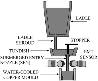
N THE continuous casting of steel [1], control of molten steel delivery through the pouring nozzle, that is, a sub-merged entry nozzle (SEN) (see Fig. 1), is critical to ensure an optimum laminar flow pattern in the casting mold and stable meniscus. The flow regime in the SEN influences the billet sur-face quality, cleanliness, and hence the value of the cast product. This is particularly important for casting low carbon aluminum killed steel as the flow profile is readily disrupted by the clog-ging problem due to the deposition of aluminum oxide particles on the inside of the SEN wall and exit ports [2], [3]. Achieve-ment of a stable and quiescent flow between the tundish andManuscript received December 19, 2003; revised October 15, 2004. This work was supported by the U.K. Engineering and Physical Sciences Research Council under Grant GR/N21055. The associate editor coordinating the review of this paper and approving it for publication was Dr. Krikor Ozanyan.
X. Ma, A. J. Peyton, and R. Binns are with the Engineering Department, Lancaster University, Lancaster LA1 4YR, U.K. (e-mail: [email protected]; [email protected]; [email protected]).
S. R. Higson is with the Corus RD&T, Teesside Technology Centre, Corus U.K., Ltd., Middlesbrough TS6 6UB, U.K. (e-mail: [email protected]).
[image:1.594.342.514.188.330.2]Digital Object Identifier 10.1109/JSEN.2004.842443
Fig. 1. Location of the submerged entry nozzle in the continuous casting process, where the position of noncontact electromagnetic sensor is also shown.
casting mold is determined by a number of interrelated casting parameters, including steel mass flow rate, tundish metal level [4], pouring nozzle diameter [2], argon gas flow rate [5], and the amount of clogging within the stopper/slide gate and pouring nozzle. Typical examples of steel flow patterns within an SEN are annular flow (a stream with a central air gap), central stream, and bubbly flow (argon bubbles with the stream) with the pos-sible transition between flow modes during casting depending on the flow rate of steel and gas for the given casting conditions. An online flow visualization approach utilizing rugged and non-invasive sensors would be highly desirable.
Much effort has been made in developing a wide variety of tomographic techniques for industrial process applications over the past two decades. For example, the use of X-rays can be considered as a proven method to visualize the flow of liquid steel [6], [7]. However, X-rays suffer from the inherent haz-ards of radiation and size of the equipment. Electrical tech-niques have received much attention recently for a number of process applications, especially online monitoring and control, thus providing inexpensive and nonintrusive imaging systems with low, but sufficient, image resolution of the internal mate-rial distributions within the processes [8], [9]. Electromagnetic inductance tomography (EMT), which requires custom data ac-quisition system and physical inductive sensors, uses magnetic coupling between sensors to provide images that represent the distributions of electrically conductive and magnetically perme-able material within the object space. This relatively new tomo-graphic technique has been researched for the similar problem of imaging molten metal solidification [10], [11]. Eddy-current techniques have also been utilized in monitoring phase trans-formation of steel samples in a hot strip mill [12] and
large steel bodies, which increase eddy currents, hence signal changes. Bubbly and annular flows can be differentiable at increased operating frequencies as bubbles in the bubbly flow impede the induced eddy-current flow at high frequencies. Previous tests have also shown that a significant reduction in the flow rate produces a partial flow in the pouring nozzle, which results in large variances in signal, as large cavities are sporadically present in the sensor space.
The design of such an instrument must consider the effects of the environment upon the sensor and hence the instrument system. The operational temperature, which varies between 1000–1500 C, demands that the sensor array should be low cost, easily maintainable, and constructed from materials capable of enduring such high temperatures. Low-input capac-itance is essential in order to maximize the resonant frequency. However, long cables, which are generally required between the sensor array and instrument during hot trails, introduce extra input capacitance, thus reducing the resonant frequency of the system. The pouring nozzle wall will induce eddy cur-rents when an alternating magnetic field is incident due to the material being electrically conductive; this affects the selection of the optimum excitation frequency.
This paper starts with an overview of electromagnetic imaging techniques. The construction of the sensor array and associated electronics are then discussed, followed by sen-sitivity map analysis and a description of the applied image reconstruction algorithm. Images, as reconstructed from cold sample measurements and hot pilot plant trials, are presented. This paper will be the first to present tomographically recon-structed images of real molten steel flows through a submerged entry nozzle. The aim of such a system is to determine, and ultimately visualize, steel flows within the SEN from which flow regime knowledge is created, thus enabling improved control over casting conditions.
II. EMT
EMT, also termed mutual inductance tomography (MIT) [16], [17], maps spatial distribution of electrical conductivity or mag-netic permeability through the measurement of magmag-netic cou-pling between inductive sensors. The underlying principle be-hind the technique can be described generally as follows: The object space is energized with a sinusoidally varying magnetic field created through excitation coils. Electrically conductive or ferromagnetic objects inside the space causes distortion to the
fore only the electrical conductivity is imaged.
For EMT, the forward problem is to predict the sensor outputs for a given material distribution with known electro-magnetic properties. Analytical approaches are suitable for solving forward problems for ideal geometries with simplified assumptions; numerical approaches, such as finite-element methods (FEM), are used to calculate approximately the forward problems in the general case. The inverse problem, through the utilization of image reconstruction techniques, is to convert the measured data into an image which represents the original material distribution. The reconstruction problem of conductivity mapping in EMT is an ill-posed and ill-condi-tioned problem as the number of pixels in an image is usually much larger than the number of the limited measurements. This problem is further complicated by the soft field effect, whereby the object material affects both the magnitude and direction of the interrogating field. Therefore, the measured induced voltage is a nonlinear function of electrical conductivity of the test objects. There is no direct approach to solving this inverse problem. It is generally necessary to use nonlinear reconstruction methods such as the regularized Gauss–Newton methods to achieve desirable images where each step in such an iterative method is treated as a regularized linear step [18].
However, assumptions are made of the system that simpli-fies the image reconstruction problem. Assuming the system to be linear so that pixel interactions are ignored, which is a very coarse approximation to reality, the system is described by a ma-trix equation
(1) where is the measurement data and the image pixel values. Vector contains elements, the total number of pixels in the object space, whereas vector contains elements, which rep-resents the total number of independent measurements, i.e., the number of unique coil pairs to be measured. The two-dimen-sional matrix of rows and columns contains the sensi-tivity coefficients, which reflect the response of each pixel to a particular measurement.
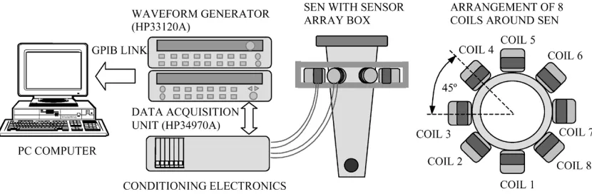
Fig. 2. Block diagram of the experimental system. The system consists of a sensor array, data acquisition unit, associated conditioning circuitry, and a PC computer, which were purposely designed and constructed for hot trials.
III. EMT IMAGINGSYSTEM
A. Experimental System
The initial investigative system based on an impedance analyzer approach proved that the use of electromagnetic approaches to visualize simple geometries was possible [14], [15]. However, an automated system is required for hot pilot plant trials. The instrument system, as schematically illustrated in Fig. 2, was designed and constructed to achieve the hot test aims. The 5-kHz 10-V ac signal is provided from a Hewlett Packard waveform generator. The conditioning electronics convert the 5-kHz voltage source to a current signal, which is driven at 300 mA to provide the coil excitation signal. The conditioning electronics also performs the demodulation of current signal and induced voltages from the detection coils with respect to excitation waveform, producing in-phase and quadrature dc components. The data acquisition unit has three tasks: the switching of the excitation signal via reed relays to each coil sequentially, control over amplitude gain selection of 1, 56, 226, and 362 depending on the detection coil posi-tion relative to excitaposi-tion coil, and converting the resolved dc components to digital signals. The data acquisition software is realized in Visual C++ making use of the Microsoft Foundation Class (MFC) library in conjunction with General Purpose Inter-face Bus (GPIB) and Virtual Instrument Software Architecture (VISA) library to facilitate nine-channel data loggings (excita-tion current and eight detec(excita-tion voltages). A Pentium-based PC computer operating the online acquisition software takes the readings via a GPIB link and stores the data in formats suitable for retrieval by software packages such as MATLAB for further imaging processing. The system has a frame acquisition rate of approximately 1.35 s.
[image:3.594.308.551.244.417.2]In order to select the optimum excitation frequency, the pen-etration effect of eddy currents into the pouring nozzle, which is typically graphite-alumina, must be considered. The elec-trical conductivity of graphite is kS/m compared to MS/m for steel at room temperature and kS/m for molten steel at 1500 C. The penetration of eddy currents into the pouring nozzle is frequency dependent. It was found that the nozzle attenuated the eddy-current signal at frequen-cies above 10 kHz. To avoid significant eddy-current losses in the nozzle walls, its operating frequency should be limited to below 10 kHz. Therefore, 5 kHz was selected as the operating
Fig. 3. Photograph of the physical sensor and nozzle model.
frequency at which the skin depth was 26.9 mm for graphite so that the nozzle had a negligible effect compared to the nozzle wall thickness (17 mm). In the meantime, the skin depth for molten steel at 1500 C was 8.0 mm, which was comparable with object space size to ensure that a sufficient volume of steel was probed.
The main sensor array components are eight coils, which were chosen as a compromise between system complexity and image resolution. Each coil was wound with copper wire (50 turns, 50-mm diameter each) and equally spaced at 45 intervals around the periphery of the SEN to preserve symmetry. Each coil, together with its associated electronics, can be multiplexed between excitation and detection tasks as directed by the PC computer. At each projection, one coil is energized while the remaining seven coils act as detectors. The quadrature signals are measured as they provide larger voltages, hence improved signal-to-noise ratio (SNR). Coils are energized in sequence to provide a total of eight projections and hence 56 measurements. However, only 28 independent measurements are used for each frame image reconstruction due to sensor coil reciprocity.
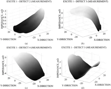
Fig. 4. Four measured primary sensitivity maps for a symmetrical eight-coil sensor array system, all dimensions inXandYdirections are in millimeters. (a) Sensitivity map for excitation coil 1 and detection coil 2. (b) Sensitivity map for excitation coil 1 and detection coil 3. (c) Sensitivity map for excitation coil 1 and detection coil 4. (d) Sensitivity map for excitation coil 1 and detection coil 5.
formers, array base, and enclosure as shown in Fig. 3, which operated at 1000 C. Silicone sealant was utilized to bond the sensor array as it also had a high temperature rating (300 C). After assembly, the coils were boxed with a central area empty to accommodate the nozzle. An air supply was applied to the en-closure passing through the coils for cooling; the internal tem-perature was monitored.
B. Sensitivity Maps
The sensitivity maps, which are dependent on the material distribution in the sensor array, show spatial sensitivity of a par-ticular excitation-detection coil combination to pixel perturba-tions within the object space. Sensitivity maps are widely used to solve the inverse problems in image reconstruction, as they describe the unique conductivity distribution to pixel perturba-tions for the given sensor array. These maps can be calculated by either analytical approximation [20], numerical approaches, or by experimental measurements. In this case, sensitivity maps were produced using direct measurements and compared with FEM simulations.
In the experimental measurements, a copper rod ( MS/m) of 12.5-mm diameter was used to represent the pixel perturbation. The rod was placed and moved upon a 10-mm grid inside the nozzle model. A square area of 49 pixels, a 7 7 matrix, was therefore required to describe the nozzle’s 70-mm diameter circular space; this required 37 individual rod positions. Only perturbations with respect to empty space were considered. The response to empty space, under identical excitation conditions, was subtracted from the outputs of a
detector coil when the target rod was present, i.e., (1) becoming ; thus, only net effects caused by the target object were recorded. To minimize the unwanted interference effects, nine scans were taken upon the detection coil voltage for each perturbation for averaging purposes. Impedance changes were calculated by dividing the averaged voltage changes and the associated current readings.
In image reconstruction, it is normally necessary to calcu-late the primary sensitivity maps due to sensor array symmetry, and all of the other maps can be derived from these by rota-tional transformations. Fig. 4 shows four primary maps for the eight-coil sensor array, which represent the changes in the imag-inary component of the mutual impedance of each coil pair. The initial maps have 37 pixels; hence, the maps have been smoothed and interpolated for adequate presentation. This process consists of a square 7 7 matrix generation from the initial 37 pixels by placing corner pixels via simple averaging of the nearest pixels, followed by both and direction interpolations onto a 200 200 pixel grid using cubic spline operations. A circular map is finally constructed using 31 415 pixels of the available 200 200 pixels. The smoothness in the shape of the maps illus-trates the minimal effect of noise upon the system. As expected, for opposite coils (1 and 5, refer to Fig. 3 for coil positions), a distinctive saddle shape is observable. The map shapes of other coil pairs (1 and 2, 1 and 3, 1 and 4; see Fig. 3) show that the increase in the magnetic field coupling is apparent when the per-turbation approaches the coils.
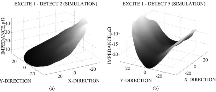
Fig. 5. Simulation sensitivity maps of coil pairs when coil 1 is excited using Maxwell (Ansoft Corporation). All dimensions inXandY directions are in millimeters. (a) Neighboring coil pairs 1 and 2 and (b) opposite coil pairs 1 and 5.
a three-dimensional (3-D) finite element package, to create the simulated sensitivity maps. This simulation software offered a piecewise solution to field problems by splitting the problem into a series of small tetrahedral elements over which the field values are approximated. A problem region was solved of five times the size of the sensor model to ensure that the applied boundary conditions did not over constrain the solution. The sur-rounding air was assigned by the material property of a vacuum. A total of 21 558 tetrahedral elements were meshed to ensure that the simulations converged to 0.5% error.
As with the experimental method, a 12.5-mm diameter copper rod was used as the target object and moved upon a 10-mm grid inside the nozzle. At each rod position, the coils were excited with a 5-kHz 300-mA sinusoidal current; Maxwell calculated the induced voltages on the sensing coils under each excitation both with and without a perturbation object inside, respectively. The time expense required for computing a full collection of 56 maps on a Pentium PC (2.20 GHz CPU, 2.0 GB RAM) was approximately 81 h. This meant that an average time of approximately 90 min was taken for one sensitivity map calculation, which was much longer than the experiment method.
Fig. 5 shows the simulated sensitivity maps, as the examples, between neighboring coil-pair (coil 1–2) and opposite coil-pair (coil 1–5). The shape similarity between the simulated and ex-perimental maps can be measured in terms of cross-correlation coefficients. Unrelated maps result in a correlation coefficient of zero, whereas equivalent maps have a correlation coefficient of one. The correlation coefficients between Figs. 4(a) and 5(a) and Figs.4(d) and 5(b) are 0.8526 and 0.8105, respectively. In addition, the normalized dot division of the simulated and exper-imental maps shows that all the dot values are between 0.5 and 1.0. All of these indicate that the simulated and experimental maps for the same coil pair are in good agreement. The differ-ences are mainly due to the significant approximations made in the simulation, for example, a single stranded turn for coils in the simulation system rather than 50 turns for coils in the real system, and the gain control, which is normally used in the instrument system for the induced voltage amplification de-pending on the coil pair position relative to the nozzle.
The final sensitivity matrix represents an amalgamation of a series of the sensitivity maps and has dimensions of 28 49,
where 28 represents elements in matrix and 49 denotes elements in matrix . An experimental sensitivity matrix was employed during image reconstruction.
C. Image Reconstruction
The SIRT reconstruction algorithm involves an iterative process to solve the equation as described in (1) for when and are known. The iterative algorithm at step is described by
(2) where represents the backward projection matrix and is the relaxation factor that controls the convergence speed of the algo-rithm. Matrix could use heavily regularized inverse matrices, for example, based on truncated singular value decomposition (SVD) [18]. However, in this case, a normalized transposition of is used, namely ( ), as it is a simplistic method for converting measurements into images. An initial guess is made for . As only conductive media is present, nonnegative constraining is used to limit the value of each pixel to lie between zero and one, where the maximum value of one corresponds to a full element and values between zero and one to partially filled elements [15].
Cold samples were initially employed to determine the ability of the system and reconstruction algorithm in distinguishing be-tween differing areas of conductivity. Titanium rods (electrical conductivity MS/m) were used as test phantoms for real problem imitation. Three titanium rods with known sizes of 19-, 25-, and 35-mm diameters were placed at different po-sitions within the nozzle. Fig. 6 shows the responses in time sequence of coil 5 acting as a detector under excitation of coil 1, as an example, to three rods at different positions. It is evi-dent that a larger rod causes larger signal changes in the induced voltage due to larger eddy-current losses. For a given phantom, the smallest signal change is found at the center position; this is in agreement with previously presented sensitivity maps. A dif-ference in signal between positions 1 and 3 for the largest rod is possible due to misalignment during these tests.
Fig. 6. Coil outputs in time sequence for small (19-mm diameter), medium (25-mm diameter), and large (38-mm diameter) rods placed at three different positions within the nozzle. Larger rod causes larger signal changes of the induced voltage due to larger eddy-current losses, and central position suffers from the least spatial resolution.
number of iterations are 0.01 and 2000, respectively, which are the case dependent. From these images, there is good accuracy between real and estimate rod positions. The relative sample size can be inferred by comparing the pixel value differences of the three rods. As a further example, Fig. 8 shows an image of three copper rods (two 19-mm-diameter rods and one small 12.5-mm-diameter rod) placed within the nozzle. The inference of the sample size becomes difficult as the magnetic field cou-pling between rods complicates the problem more than in the single-rod case. However, the position predictions are in good agreement with the real positions.
IV. HOTPLANTTRIALRESULTS
Hot casting trials were undertaken using the heavy pilot plant facilities at Corus Teesside Technology Centre. The trial arrangement is shown in Fig. 9. The sensor array was placed around a transparent quartz glass tube, which was positioned off center (top right), within a standard slab caster SEN and connected to the EMT instrument through long thermally shielded cables, which suffered no degradation of signal over the required 7 m. Molten steel was supplied from a 4-ton nominal capacity electric arc furnace via a stoppered ladle to a tundish and then passed to a pseudo-casting mold via the glass tube to enable submerged pouring to be simulated. Two scans were taken for averaging purposes, which resulted in a sampling rate of 2.70 s/frame. Casting was maintained for approximately 220 s. During data loggings, flow patterns were also observed and recorded using video.
Fig. 10 shows the sensor outputs throughout casting for the cases of a neighboring coil-pair (coil 1–2) and an opposite coil-pair (coil 1–5). The short step changes of the detected signal are the indicators of casting commencing and casting stopping during pouring. Two breaks in casting are observed in the illustration, which were manually established by controlling
Fig. 7. Images of small (19-mm diameter), medium (25-mm diameter), and large (38-mm diameter) titanium rods: (a) small rod at (0,0), (b) medium rod at (020,0), and (c) large rod at (20,0).
[image:6.594.40.290.63.273.2]Fig. 8. Images of two copper rods (19-mm diameter at (020, 10) and (10,
010), respectively) and one small copper rod [12.5-mm diameter at (20, 10)] when placed within nozzle simultaneously.
Fig. 9. Hot casting trials using the pilot plant facilities at Corus Teesside Technology Centre.
achieve a thermal-free signal. All sensor outputs are treated accordingly to remove thermal effects.
[image:7.594.305.554.64.513.2]The thermally compensated outputs are arranged in a matrix such that the rows represent the time sequence, i.e., image frame index, and the columns the coil-pair measurements respectively. Images of steel flow profiles are then produced by utilization of the reconstruction algorithm with iterations and nonnegative constraining. More iterations are used due to a reduction in the SNR of hot trial signals. A selection of results is shown in Fig. 11. The images are shown in sequence from left to right and then top to bottom with a common gray scale. All images adequately predict the position, i.e., the upper right side of the SEN. The two breaks in the pour at approximately 65 and 140 s are clearly visible. The changes of steel flow profiles can
Fig. 10. Display of the detected signals during hot trial and thermal drift effect removal: (a) coil 2 excited by coil 1 and (b) coil 5 excited by coil 1.
be differentiated in terms of the variation in grey level which lies at the right of each image.
It is evident that these images provide a good representation of the steel flow profile changes through the SEN during casting. The results were consistent with video recording of an exposed section of the steel flow. Consequentially, the hot trial results demonstrate that the electromagnetic sensing technique can be used to monitor and visualize the real molten steel flow through a pouring nozzle.
V. CONCLUSION
[image:7.594.44.285.288.550.2]Fig. 11. Images of molten steel flow profiles through the SEN during hot trial at different time instants; two stops are also included (black images). Changes of steel flow profiles can be differentiated in terms of the variation in grey level which lies at the right of each image.
system, at which the conductive nozzle has little effect upon field penetration. Images from the cold sample tests show that the object position can be discriminated and the inference of the relative object size is possible. The promising results from the preliminary pilot plant trials demonstrate that the EMT ap-proach can be utilized to monitor and visualize real molten steel flow through a pouring nozzle.
The present system uses a simple reconstruction algorithm for image reconstruction and has a low data acquisition rate (1.35 s per frame). An improved EMT system is under development to increase acquisition speed, decrease system size, improve reso-lution, and present the images in real time. An improved recon-struction algorithm, based on nonlinear regularised techniques, such as Gauss–Newton methods, is also being formulated for hot trial measurement data. Also, as single frequency excitation has been shown to inadequately resolve complex flow regimes, a multifrequency measurement approach and a subsequent in-version algorithm is required to offer a solution capable of vi-sualizing complex annular and bubbly flows within the nozzle. Nevertheless, it is believed that the EMT application holds sig-nificant promise for the future industrial process.
ACKNOWLEDGMENT
The authors would like to thank M. Chamberlain for his con-tributions during this work and Dr. W. D. N. Pritchard of Corus, U.K., Ltd. for his help and support during hot trials.
REFERENCES
[1] X. Ma, A. J. Peyton, R. Binns, and S. R. Higson, “Imaging the flow profile of molten steel through a submerged pouring nozzle,” inProc. 3rd World Congr. Industrial Process Tomography, Banff, AB, Canada, 2003, pp. 736–742.
[2] F. G. Wilson, M. J. Heesom, A. Nicholson, and A. W. D. Hills, “Effect of fluid flow characteristics on nozzle blockage in aluminum killed steels,”
Ironmaking Steelmaking, vol. 14, pp. 296–309, 1987.
[3] H. Yin, H. Shibata, T. Emi, and M. Suzuki, “Characteristics of agglom-eration of various inclusion particles on molten steel surface,”Iron Steel Inst. Japan Int., vol. 37, pp. 946–955, 1997.
[4] F. L. Kemeny, “Tundish nozzle clogging: Measurement and prevention,” inProc. Mclean Symp., 1998, pp. 103–110.
[5] H. Bai and B. G. Thomas, “Effects of clogging, argon injection and con-tinuous casting conditions on flow and air aspiration in submerged entry nozzles,”Metallurg. Mater. Trans. B, vol. 32, pp. 707–722, 2001. [6] M. Hytros, I. Jureidini, D. Kim, J. H. Chun, R. Lanza, and N. Saka,
“A computed tomography sensor for solidification monitoring in metal casting,” inProc. TMS Annu. Meeting Materials Processing, 1997, pp. 173–181.
[7] M. Hytros, I. Jureidini, J. H. Chun, R. Lanza, and N. Saka, “High-energy x-ray computed tomography of the progression of the solidification front in pure aluminum,”Metallurg. Mater. Trans. A, vol. 30, pp. 1403–1410, 1999.
[8] W. Q. Yang, A. L. Stott, M. S. Beck, and C. G. Xie, “Development of ca-pacitance tomographic imaging systems for oil pipeline measurements,”
Rev. Sci. Instrum., vol. 66, pp. 4326–4332, 1995.
[9] M. Wang, A. Dorward, D. Vlaev, and R. Mann, “Measurements of gas-liquid mixing in a stirred vessel using electrical resistance tomography (ERT),”Chem. Eng. J., vol. 77, pp. 93–98, 2000.
[10] M. H. Pham, Y. Hua, and N. Gray, “Imaging the solidification of molten metal by eddy currents – Part 1,”Inv. Probl., vol. 16, pp. 469–482, 2000. [11] , “Imaging the solidification of molten metal by eddy
cur-rents—Part 2,”Inv. Probl., vol. 16, pp. 483–494, 2000.
[12] S. Johnstone, R. Binns, A. J. Peyton, and W. D. N. Pritchard, “Using electromagnetic methods to monitor the transformation of steel sam-ples,”Trans. Instrum. Meas. Contr., vol. 23, pp. 21–29, 2001. [13] K. P. Dharmasena and H. N. G. Wadley, “Eddy current sensor concepts
for the Bridgman growth of semiconductors,”J. Crystal Growth, vol. 172, pp. 303–312, 1997.
[14] R. Binns, A. R. A. Lyons, and A. J. Peyton, “Imaging of steel profiles within a pouring nozzle,” inProc. 2nd World Congr. Industrial Process Tomography, Hanover, Germany, 2001, pp. 138–145.
[15] R. Binns, A. R. A. Lyons, A. J. Peyton, and W. D. N. Pritchard, “Imaging molten steel flow profiles,”Meas. Sci. Technol., vol. 12, pp. 1132–1138, 2001.
[16] A. J. Peyton, Z. Z. Yu, G. Lyon, S. Al-Zeibak, J. Ferreira, J. Velez, F. Linhares, A. R. Borges, H. L. Xiong, N. H. Saunders, and M. S. Beck, “An overview of electromagnetic inductance tomography: Description of three different systems,”Meas. Sci. Technol., vol. 7, pp. 261–271, 1996.
[18] W. R. B. Lionheart, “Reconstruction algorithms for permittivity and con-ductivity imaging,” inProc. 2nd World Congr. Industrial Process To-mography, Hanover, Germany, 2001, pp. 4–11.
[19] A. R. Borges, J. E. Oliverira, J. Velez, C. Tavares, F. Linhares, and A. J. Peyton, “Development of electromagnetic tomography (EMT) for indus-trial applications, Part 2: Image reconstruction and software framework,” inProc. 1st World Congr. Industrial Process Tomography, Buxton, U.K., 1999, pp. 219–225.
[20] A. J. Peyton, S. Watson, R. J. Williams, H. Griffiths, and W. Gough, “Characterising the effects of the external electromagnetic shield on a magnetic induction tomography sensor,” inProc. 3rd World Congr. In-dustrial Process Tomography, Banff, Canada, 2003, pp. 352–357.
Xiandong Mareceived the B.Eng. degree in elec-trical engineering from Jiangsu University of Science and Technology, China, in 1986, the M.Sc. degree in power systems and automation from Nanjing Au-tomation Research Institute (NARI), China, in 1989, and the Ph.D. degree in partial discharge detection and analysis from Glasgow Caledonian University, U.K., in 2003.
Between 1989 and 1998, he worked with NARI as an Electrical Engineer for eight years and later as a Senior Engineer for two years, developing DSP-based power system real-time digital simulators dedicated for close-loop power equipment testing. He has been a Research Associate at Lancaster University, Lancaster, U.K., since 2002, and his current research interests include electro-magnetic induction tomography for industrial process, nondestructive testing, and instrumentation.
Anthony J. Peytonreceived the B.Sc. (first class) degree in electrical engineering and electronics and the Ph.D. degree from the University of Manchester Institute of Science and Technology (UMIST), Man-chester, U.K., in 1983 and 1986, respectively.
He was appointed a Principal Engineer at Kratos Analytical, Ltd., in 1989, developing precision electronic instrumentation systems for the magnetic sector and quadrupole mass spectrometers, from which an interest in electromagnetic instrumentation developed. He returned to UMIST as a Lecturer and worked with the Process Tomography Group. He moved to Lancaster University, Lancaster, U.K., with his research team, in 1996, as a Senior Lecturer. He was promoted to Reader in electronic instrumentation in July 2001 and to Professor in May 2004. His main research interests include the areas of instrumentation, applied sensor systems, and electromagnetics.
Richard Binnsreceived the M.Eng. degree in mechatronics and the Ph.D. de-gree from Lancaster University, Lancaster, U.K., in 1998 and 2002, respectively. After working for 18 months at a defense company, which specialized in radar products, he accepted a Research Associate position at Lancaster University. He is currently investigating the implications of using ultrawide-band radar to detect and image various materials and geometries.

![Fig. 8.Images of two copper rods (19-mm diameter at (�20, 10) and (10,�10), respectively) and one small copper rod [12.5-mm diameter at (20, 10)]when placed within nozzle simultaneously.](https://thumb-us.123doks.com/thumbv2/123dok_us/7988723.758769/7.594.305.554.64.513/images-copper-diameter-respectively-copper-diameter-placed-simultaneously.webp)

