The driving force of labor productivity

Munich Personal RePEc Archive

The driving force of labor productivity

Kitov, Ivan and Kitov, Oleg

Institute for the Geospheres’ Dynamics, University of Warwick

10 June 2008

Online at

https://mpra.ub.uni-muenchen.de/9069/

The driving force of labor productivity

Ivan O. Kitov & Oleg I. Kitov

Abstract

Labor productivity in developed countries is analyzed and modeled. Modeling is based on our previous finding that the rate of labor force participation is a unique function of GDP per capita. Therefore, labor productivity is fully determined by the rate of economic growth, and thus, is a secondary economic variable.

Initially, we assess a model for the U.S. and then test it using data for Japan, France, the UK, Italy, and Canada. Results obtained for these countries validate those for the U.S. The evolution of labor force productivity is predictable at least at an 11-year horizon.

JEL classification: J2, O4

Introduction

Mainstream economics sees labor productivity as the central problem for the understanding of

economic evolution. An elevated rate of the growth in labor productivity in the 1990s was

considered by Blinder and Yellen (2002) as the driving force of the excellent economic

performance. Correspondingly, a slightly lowered growth rate in the 1970s was responsible for

“the woeful macroeconomic performance of that decade”. Bearing in mind the importance of

labor productivity for theoretical and practical purposes, we would like to answer two basic

questions:

1. What is the driving force behind the growth of labor productivity?

2. Is it possible to control this force and to achieve stable economic growth?

Quantitative answers to these questions would allow elaboration of a set of reasonable policies in

many areas aimed at the acceleration of real economic growth.

From our previous experience with analyzing and modeling real economic growth,

among numerous aspects associated with the study of labor productivity, we are specifically

interested in its link to the growth in real GDP per capita and to labor force participation rate. For

example, Campbell (1994) and Pakko (2002) reported that a decrease in the growth rate of

productivity rate results in increasing in employment and output. In several working papers

(Kitov, 2006ab; Kitov, Kitov, and Dolinskaya, 2007a) we demonstrated that the evolution of real

GDP per capita in the USA is driven by the change in the number of 9-year-olds. In turn, Kitov

and Kitov (2008) found that the evolution of labor force participation rate is controlled by real

GDP per capita as the only driving force. By definition, labor productivity is a ratio of real GDP

and the number of employed persons (or the number of worked hours). Hence, the growth in

productivity is also driven by the only macroeconomic variable – real GDP per capita (or the

change in the specific age population).

Conventional economics includes extensive literature devoted to the understanding and

modeling of the forces (beyond that we investigate here) behind real economic growth.

Handbook of Economic Growth (2005) is a valuable source of relevant information and

references. Since we are focusing on the aforementioned links in this paper, we explain long- and

mid-term trends as well as short-term fluctuations in labor productivity using only real economic

growth. Our analysis for the USA is supported and validated by a cross-country comparison.

The remainder of the paper is organized as follows. Section 1 presents some working

assumptions and quantitative relationships between labor productivity, labor force participation

these relationships against actual data and present some predictions of the future evolution of

productivity in the USA. Section 3 extends our analysis to some other developed countries.

Section 4 concludes.

1. The model

For the estimation of (average) labor productivity, P, one needs to know total output, GDP, and

the level of employment, E (P=GDP/E), or total number of working hours, H (P=GDP/H). First

definition includes employment, which is usually determined in the Current Population Surveys

conduced at a monthly rate by the U.S. Census Bureau. In the first approximation and for the

purposes of our modeling, we neglect the difference between the employment and the level of

labor force because the number of unemployed is only a small portion of the labor force. There is

no principal difficulty, however, in the subtraction of the unemployment, which is completely

defined by the labor force level with possible complication in some countries induced by time

lags (Kitov, 2006cd, Kitov, Kitov, and Dolinskaya, 2007b). Hence, a more accurate relationship

between productivity and real GDP per capita is potentially available.

The number of working hours is an independent measure of the workforce. Employed

people do not have the same amount of working hours. Therefore, the number of working hours

may change without any change in the level of employment and vice versa. In this study, the

estimates associated with H are used as an independent measure of productivity and for

demonstration of the inherent uncertainty in definitions of labor productivity.

Obviously, individual productivity varies in a wide range in developed economies. In

order to obtain a hypothetical true value of average labor productivity one needs to sum up

individual productivity of each and every employed person with corresponding working time.

This definition allows a proper correction when one unit of labor is added or subtracted and

distinguishes between two states with the same employment and hours worked but with different

productivity. Hence, both standard definitions are slightly biased and represent approximations

to the true productivity. Due to the absence of true estimates of labor productivity and related

uncertainty in the approximating definitions we do not put severe constraints on the precision in

our modeling and seek only for a visual fit between observed and predicted estimates.

Real GDP in the definitions of labor productivity is a measured macroeconomic variable.

There is no need to model it in this study and we use the estimates reported by the Bureau of

Economic Analysis (BEA). Second term (E or H) in the definitions can be and is actually

measured. At the same time, it has been definitely driven by one exogenous variable since the

mid-1960s. Recently, we developed a model (Kitov and Kitov, 2008) describing the evolution of

variable – real GDP per capita, G. Natural fluctuations in real economic growth unambiguously

lead to relevant changes in labor force participation rate as expressed by the following

relationship:

{B1dLFP(t)/LFP(t) + C1}exp{ α1[LFP(t) - LFP(t0)]/LFP(t0) =

= {dG(t-T))/G(t-T) – A1/G(t-T)}dt (1)

where B1 and C1 are empirical (country-specific) calibration constants, α1 is empirical (also

country-specific) exponent, t0is the start year of modeling, T is the time lag, and dt=t2-t1, t1 and

t2 are the start and the end time of the time period for the integration of g(t) = dG(t-T))/G(t-T) –

A1/G(t-T) (one year in our model). Term A1/G(t-T), where A1 is empirical constant, represents the

evolution of potential economic growth (Kitov, 2006b). The exponential term defines the change

in the sensitivity to G due to deviation of the LFP from its initial value LFP(t0). Relationship (1)

fully determines the behavior of the LFP when G is an exogenous variable.

It follows from (1) that productivity can be represented as a function of LFP and G,

P~G N/N LFP = G/LFP, where N is the working age population. Hence, P is a function of G

only. Therefore, the growth rate of labor productivity can be represented using several

independent variables. Because the change in productivity is synchronized with that in G and

labor force participation, first useful form mimics (1):

dP(t)/P(t) = {B2dLFP(t)/LFP(t) + C2}·exp{ α1[LFP(t) - LFP(t0)]/LFP(t0)} (1 )

where B2 and C2 are empirical calibration constants. Inherently, the participation rate is not the

driving force of productivity, but (1 ) demonstrates an important feature of the link between P

and LFP – the same change in the participation rate may result in different changes in the

productivity depending on the level of the LFP.

In order to obtain a simple functional dependence between P and G one can use two

alternative forms of (1), as proposed by Kitov and Kitov (2008):

{B3dLFP(t)/LFP(t) + C3} exp{α2[LFP(t) - LFP(t0)]/LFP(t0)} = N9(t-T)

dP(t)/P(t) = B4N9(t-T)+ C4 (2)

where N9 is the number of 9-year-olds, B3,…, C4 are empirical constant different from B2, C2, and

driven by the change rate of the number of 9-year-olds (specific age for U.S. population).

Relationship (2) links dP/P and N9 directly.

The next relationship defines dP/P as a nonlinear function of G and serves a workhorse

for those countries, which do not provide accurate estimates of specific age population. General

nonlinear dependence between P and G is as follows:

N(t2) = N(t1)·{ 2[dG(t2-T)/G(t2-T) - A2/G(t2-T)] + 1} (3)

dP(t2)/P(t2) = N(t2-T)/B + C (4)

where N(t) is the (formally defined) specific age population, as obtained using A2 instead of A1, B

and C are empirical constants. Relationship (3) defines the evolution of some specific age

population, which is different from actual one. This discrete form is useful for calculations.

So, there are three different relationships to test. We use a simplified form of testing

procedure - visual fit between measured and predicted rate of productivity growth. The estimates

of goodness-of-fit obtained using linear regression analysis are facultative ones.

2. Modeling the evolution of productivity in the U.S.

There are several sources of productivity estimates. We use the estimates reported by the

Conference Board (2008) and the Bureau of Labor Statistics (2008). Our model predicts the

change rate of labor productivity. The upper panel in Figure 1 presents four time series which

correspond to two different definitions of productivity. Two curves represent output in U.S.

dollars per one hour (ratio of total output and total working hours in the USA). Other two curves

represent output per employed person per year. These four curves span the period between 1960

and 2007 and demonstrate similar overall behavior with a deep trough around 1980. Also, notice

a decline in productivity since 2003 for all definitions.

Amplitudes of fluctuations clearly differ between the curves. Output per person is

characterized by a slightly higher volatility. Due to the observed uncertainty in definitions and

measurements one should not expect any model to precisely reproduce these curves. The lower

panel depicts the original time series smoothed by a centered 5-year moving average, MA(5).

Only output per person estimated by the BLS still has negative values near 1980.

At first, we test our basic hypothesis that the evolution of labor force participation can

define that of labor productivity. As discussed above, we replace employment, E, in the

definition of productivity with LFP. Thus, one has to estimate coefficients B2, C2, and 1, which

curves reported by the BLS (both GDP/E and GDP/H) and those predicted with B2= -5.0,

C2=0.040, and 1=5.0; and B2= -3.5, C2=0.042, and 1=3.8, respectively. Due to volatility in the

original productivity and labor force (time derivative) series we replace them with their MA(5).

A five-year-long time interval provides an increased resolution and allows smoothing

measurement noise. As expected, coefficient B2 is negative implying a decline in productivity

with increasing labor supply. Both exponents 1 are positive. According to (1 ), this fact

indicates that the sensitivity of productivity to changes in labor force participation (or to real

economic growth) increases with the level of LFP. The goodness-of-fit for both observed time

series is about (R2=) 0.6. Moreover, principal features (troughs and peaks) of the observed series

are similar in the predicted series, with small time shifts, however. One can approximately divide

the whole period into two segments - before and after 1990. In these segments, the predicted

curves lag behind and lead the observed ones, respectively.

As in our previous paper (Kitov and Kitov, 2008), the number of 9-year-olds is obtained

from the Census Bureau (2008). [Also, we use here the estimates of real GDP per capita (in 1990

U.S. dollars converted at Geary Khamis PPPs) as presented by the Conference Board (2008).]

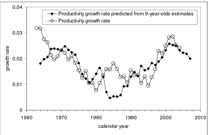
These population estimates allow to model labor productivity as defined by (2). Figure 3

compares the BLS (per hour) labor productivity and that obtained using (2) with the following

coefficients: B3=48000000, C3=-0.062, and T=2 years. The overall fit is reasonably good with

R2=0.46. There is a period of large discrepancy between the observed and predicted curves in the

mid-1980s. As with labor force participation, the predicted time series leads the observed one by

2 years.

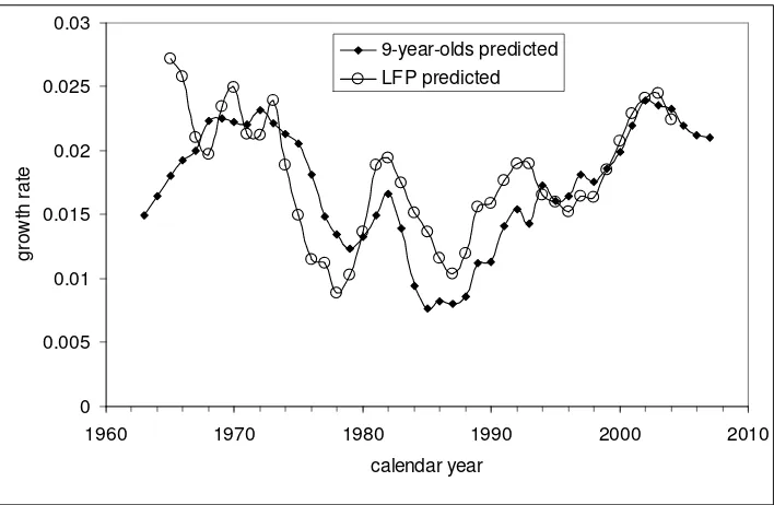
Figure 4 compares two different predictions of productivity: the one obtained from the

LFP and that from the N9. The LFP predicted curve is smoothed with MA(5) and that from N9 is

obtained with original annual readings. The agreement between these two curves is slightly

better than their agreement with the measured productivity curves. This better agreement might

be related to the fact that both predictions are associated with population estimates and the

productivity is estimated using real GDP reported by the BEA. Revisions to these different time

series might be not synchronous and create time shifts in the curves. Problems induced by

numerous revisions to population and GDP time series deserve more attention.

Relationship (2) provides a unique opportunity to predict the evolution of productivity at

an 11-year-long time horizon. The number of 9-year-olds can be extrapolated 9 years ahead

using population estimates in younger cohorts. Additional 2 years are related to the time lag

between real economic growth and productivity change. Figure 5 presents population estimates

for 9-, 6- and 1-year-olds as published by the U.S. Census Bureau (2008). The curves for

estimates of 9-year-olds. The level of the curves increases with time due to positive overall

migration, i.e. the number of 9-year-olds in a given year is the number of 1-year-olds 8 years

before plus net migration less total deaths. We are interested in the change rate of N9, however.

The lower panel in Figure 5 demonstrates that the estimates of the change rate are very close for

all three cohorts, except some short periods, where revisions to these series were different. This

closeness implies that one can replace the change rate of N9 8 years ahead with the current

change rate of the number of 1-year-olds. Hence, productivity in the USA will grow at an

elevated (relative to potential) rate during the 2010s. This process will be obviously

accompanied by an associated decrease in the LFP. If the population estimates are accurate, one

can expect sharp changes in real economic growth, labor force participation, and thus, in

productivity.

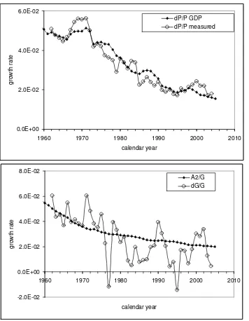
Relationships (3) and (4) define productivity as a function of real economic growth.

Figure 6 shows the difference between real GDP per capita and productivity. (Linear regression

gives the goodness-of-fit of R2=0.61.) The productivity varies with lower amplitudes because

employment is synchronized with the evolution of G and total population does not depend on G.

Two potential growth rates related to G and P are also shown: A1/G and A2/G, where A1=$420

and A2=$398. The potential rate of real economic growth is slightly higher than that for

productivity. Both constants are determined with high accuracy because even small deviations in

the rates results in large deviations in cumulative growth. Therefore, the difference between A1

and A2 is significant despite the curves are so close. The observed productivity curve was below

its potential between 1965 and 1982. As compensation, this period is characterized by intensive

growth in labor force participation. Since 1982, the productivity fluctuates around its potential.

Results of productivity modeling by (3) and (4) are presented in Figure 7. (Model

parameters are given in Figure captions.) Overall, 60% of variability in observed curve is

explained by the predicted one – same as explained by G itself. Timing of main turns in the

curves is excellent. This is an expected effect, however, because productivity is essentially the

same class variable as real GDP per capita. An important feature to predict is amplitude, as

Figure 6 indicates - productivity is not a scaled version of real GDP per capita. So, the success of

our model is related to a good prediction of LFP. Modeling of the evolution of productivity for

other developed countries using relevant GDP per capita is necessary to validate our model.

3. Modeling labor productivity in developed countries

In this Section, we use only relationship (3) and (4) for the prediction of labor productivity in a

number of developed countries. Essentially, these are the countries for which we modeled labor

developed economies in the world. The evolution of productivity in Germany is not modeled

because of side effects induced by the reunification in the 1990s.

The upper panel in Figure 8 presents observed and predicted productivity growth rate in

France. It has been decreasing from 0.05 y-1 in the 1960s to 0.02 y-1 in the 2000s. This is the

result of real economic growth below its (relatively high) potential rate defined by A2=$450, as

the lower panel in Figure 8 demonstrates. Both productivity curves are well synchronized but are

non-stationary. This might make problematic the results of linear regression analysis with

R2=0.91 due to a possibility of spurious regression. However, both variables include real GDP as

the main part. Hence, high correlation between them is not a surprise. All in all, the predicted

curve is in excellent agreement with the observed one and this observation confirms the results

for the USA and supports our model.

Figure 9 depicts observed and predicted productivity for Italy. These curves are similar to

those for France and are also in an excellent agreement: the goodnessoffit is also very high

-(R2=) 0.9. The range of productivity change for Italy is even larger: from 0.08 y-1 in the 1960s to

0.0 y-1 in the 2000s. Hence, real economic growth has been far below its potential rate since

1960s. The current rate of productivity growth is very low and one should not expect any break

in the declining trend. The growth rate of labor force has been hovering around zero line since

the mid-1970s.

The case of Canada adds some new features to our analysis. Figure 10 displays measured

and predicted rate of productivity growth. The curves are very close with R2=0.8, but are

characterized by the presence of three peaks – in the early 1960s, between 1983 and 1987, and

around 1995. This pattern is quite different from that observed in the USA – the closest neighbor

and main trade partner. So, real economic evolution in Canada and U.S. is likely to be

independent. For Canada, the range of productivity change is smaller than that in France and

Italy: from 0.03 y-1 in the 1960s to 0.0 y-1 in 1980. The current rate of productivity growth is also

close to 0.

United Kingdom and Japan are presented in Figure 11 and 12, respectively. They are

similar in sense that accurate prediction from G is possible only after 1970. The predicted curves

describe amplitudes and timing of major turns in the observed curves. The discrepancy before

1970 is not well explained and might be linked to revisions to employment and real economic

growth definitions and measurement errors.

4. Conclusion

In Introduction, we formulated two general questions. To answer the first of them, we have

Japan, the UK, France, Italy, and Canada. With a varying level of success, the growth rate of

productivity is explained by the influence of a single driving force – real GDP per capita. As a

dependent variable, labor productivity can be predicted at various time horizons with the

uncertainty determined only by the accuracy of population estimates.

The answer to the second question is – "yes". Productivity, as an economic variable, is of

a secondary importance. The growth of GDP per capita above or below its potential rate, as

defined by the term A2/G, is transferred one-to-one in relevant changes in labor force

participation and, thus, in employment and productivity. Since real economic growth depends

only on the evolution of specific age population, one must control demographic processes in

order to control productivity and stable economic growth.

One may also conclude that all attempts to place labor productivity in the center of

conventional theories of real economic growth are practically worthless. Productivity is not an

References

Blinder, A. , Yellen, J., (2002). The Fabulous Decade: Macreconomic Lessons from the 1990s. In: A.B. Krueger and R.M. Solow (eds.) The Roaring 1990s: Can Full Employment Be Sustained? New York: Russel Sage Foundation, 2002.

Bureau of Labor Statistics, (2008). Productivity and Costs, retrieved from http://data.bls.gov/cgi-bin/surveymost?pr, March 30, 2008.

Campbell, J.Y., (1994). Inspecting the Mechanism: An Analytical Approach to the Stochastic Growth Model. Journal of Monetary Economics 33(3), June 1994, 463-506.

Census Bureau, (2008). Table. Population estimates, retrieved from http://www.census.gov/popest/estimates.php, March 30, 2008.

Conference Board, (2008). Total Economy Database, retrieved from http://www.conference-board.org/economics/database.cfm, March 30, 2008.

Handbook of Economic Growth, (2005). P. Aghion and S. Durlauf (eds.), Elsevier.

Kitov, I., (2006a). GDP growth rate and population, Working Papers 42, ECINEQ, Society for the Study of Economic Inequality, http://ideas.repec.org/p/inq/inqwps/ecineq2006-42.html

Kitov, I., (2006b). Real GDP per capita in developed countries, MPRA Paper 2738, University Library of Munich, Germany, http://ideas.repec.org/p/pra/mprapa/2738.html

Kitov, I. (2006c). Inflation, unemployment, labor force change in the USA, Working Papers 28, ECINEQ, Society for the Study of Economic Inequality,

http://ideas.repec.org/p/inq/inqwps/ecineq2006-28.html

Kitov, I., (2006d). Exact prediction of inflation in the USA, MPRA Paper 2735, University Library of Munich, Germany, http://ideas.repec.org/p/pra/mprapa/2735.html

Kitov, I., Kitov, O., (2008). The driving for of labor force participation rate, MPRA Paper 8677, University Library of Munich, Germany, http://ideas.repec.org/p/pra/mprapa/8677.html

Kitov, I., Kitov, O., Dolinskaya, S., (2007a). Modelling real GDP per capita in the USA: cointegration test, MPRA Paper 2739, University Library of Munich, Germany,

http://ideas.repec.org/p/pra/mprapa/2739.html

Kitov, I., Kitov, O., Dolinskaya, S., (2007b). Inflation as a function of labor force change rate: cointegration test for the USA, MPRA Paper 2734, University Library of Munich, Germany, http://ideas.repec.org/p/pra/mprapa/2734.html

Figures

-0.04 -0.02 0 0.02 0.04 0.06

1950 1960 1970 1980 1990 2000 2010

calendar year

g

ro

w

th

r

a

te

BLS - per hour BLS - per person

CB - per hour CB - per person

-0.02 0 0.02 0.04

1950 1960 1970 1980 1990 2000 2010

calendar year

g

ro

w

th

r

a

te

MA(5) - BLS per hour MA(5) - BLS per person MA(5) - CB per hour MA(5) - CB per person

a)

-0.01 0 0.01 0.02 0.03 0.04

1960 1970 1980 1990 2000 2010

calendar year

g

ro

w

th

r

a

te

MA(5) - BLS per person predicted - LFP

b)

0 0.01 0.02 0.03 0.04

1960 1970 1980 1990 2000 2010

calendar year

g

ro

w

th

r

a

te

MA(5) - BLS per hour predicted - LFP

Figure 2. Observed and predicted growth rate of labor productivity. Two BLS measures of productivity are presented: a) output ($) per person ; b) output ($) per hour.

0 0.01 0.02 0.03 0.04

1960 1970 1980 1990 2000 2010

calendar year

g

ro

w

th

r

a

te

Productivity growth rate predicted from 9-year-olds estimates Productivity growth rate

0 0.005 0.01 0.015 0.02 0.025 0.03

1960 1970 1980 1990 2000 2010

calendar year

g

ro

w

th

r

a

te

9-year-olds predicted LFP predicted

a)

3.5E+06 4.0E+06 4.5E+06

1990 1995 2000 2005 2010 2015 2020

calendar year # 1- year-olds 6- year-olds 9- year-olds b) -0.04 -0.02 0 0.02 0.04 0.06 0.08

1990 1995 2000 2005 2010 2015 2020

calendar year c h a n g e r a te 1- year-olds 6- year-olds 9- year-olds

Figure 5. Prediction of the number of 9-year-olds by extrapolation of population estimates for younger ages (1- and 6-year-olds).

a) Total population estimates. The time series for younger ages are shifted ahead by 8 and 3 years, respectively.

b) Change rate of the population estimates, which is proportional to the growth rate of real GDP per capita. Notice the difference in the change rate provided by 1-year-olds and 6-year-olds for the period between 2003 and 2010. This discrepancy is related to the age-dependent difference in population revisions.

-4.0E-02 -2.0E-02 0.0E+00 2.0E-02 4.0E-02 6.0E-02 8.0E-02

1960 1970 1980 1990 2000 2010

calendar year

g

ro

w

th

r

a

te

dG/G dP/P A2/G A1/G

-2.0E-02 0.0E+00 2.0E-02 4.0E-02

1960 1970 1980 1990 2000 2010

calendar year

g

ro

w

th

r

a

te

predicted from GDP per capita MA(5) - CB per person

Figure 7. Observed and predicted change rate of productivity (Conference Board GDP per person employed). The observed curve is represented by MA(5) of the original one. Linear regression gives R2=0.6.

0.0E+00 2.0E-02 4.0E-02 6.0E-02

1960 1970 1980 1990 2000 2010

calendar year

g

ro

w

th

r

a

te

dP/P GDP dP/P measured

-2.0E-02 0.0E+00 2.0E-02 4.0E-02 6.0E-02 8.0E-02

1960 1970 1980 1990 2000 2010

calendar year

g

ro

w

th

r

a

te

A2/G dG/G

Figure 8. Upper panel: observed and predicted productivity in France. Model parameters:

N(1959)=570000, A2=$450, B=7500000, C=-0.022. R

2

-2.0E-02 0.0E+00 2.0E-02 4.0E-02 6.0E-02 8.0E-02 1.0E-01

1960 1970 1980 1990 2000 2010

calendar year

g

ro

w

th

r

a

te

dP/P GDP dP/P measured

-2.0E-02 0.0E+00 2.0E-02 4.0E-02

1960 1970 1980 1990 2000 2010

calendar year

g

ro

w

th

r

a

te

dP/P GDP dP/P measured

0.0E+00 1.0E-02 2.0E-02 3.0E-02 4.0E-02 5.0E-02 6.0E-02 7.0E-02 8.0E-02

1960 1970 1980 1990 2000 2010

calendar year

g

ro

w

th

r

a

te

dP/P GDP dP/P measured

-2.0E-02 0.0E+00 2.0E-02 4.0E-02 6.0E-02 8.0E-02 1.0E-01 1.2E-01

1960 1970 1980 1990 2000 2010

calendar year

g

ro

w

th

r

a

te

dP/P GDP dP/P measured

Figure 12. Observed and predicted productivity in Japan: N(1959)=2000000, A2=$400,