Analyzing repeated-game economics
experiments: robust standard errors for
panel data with serial correlation
Vossler, Christian A.
Department of Economics and Howard H. Baker Jr. Center for
Public Policy, University of Tennessee
January 2009
Analyzing Repeated-Game Economics Experiments: Robust Standard Errors
for Panel Data with Serial Correlation
Christian A. Vossler
1. Introduction
Many laboratory and field experiments in economics involve participants or groups of
participants making a sequence of related decisions, usually with feedback, over many choice
periods. For instance, this is typical of experimental work on auctions, bargaining, the private
provision of public goods, tax compliance, and pollution control instruments. Through
repeated-game play, researchers allow for developments such as learning, strategy refinement,
establishment of equilibria, and observances of how decisions or outcomes change in response to
experimental design variations. The widespread availability and improving functionality of
computer software has made it increasingly common for experiments to be reasonably complex
and involve many choice periods.
Experimentalists traditionally have relied on fairly simple and computationally
transparent parametric and nonparametric hypothesis tests to evaluate hypotheses (e.g. paired t
-test, Wilcoxon test), such as those discussed in Davis and Holt (1993). It remains a somewhat
common practice to address the time-series dimension superficially by using as the unit of
observation the mean outcome across all periods for an individual or group. Time trends may be
artificially accounted for by using the average outcome from the last decision period, last few
periods, or by separately testing different period groupings. Such analyses rely on the variation in
means across individuals or groups and insufficiently accounts for the variation in outcomes
across decision periods. These approaches are particularly troublesome for experimental designs
Particularly in the last several years, experimentalists have relied more on available
estimation methods for panel data.1 These methods include standard random effects (or closely
related mixed effects) and fixed effects models, as well as the use of common estimators for
cross-section data (e.g. OLS) in tandem with “robust” covariance matrix estimators such as
White’s (1980) heteroskedasticity-consistent estimator and Beck and Katz’s (1995)
“panel-corrected standard errors”. While these approaches allow analysis of the full data set while
accounting for important forms of heterogeneity, they may inadequately address inference issues
related to serial correlation. In some instances where serial correlation has been explicitly
addressed in experimental analyses, convenient parametric modeling approaches have been
employed, such as the inclusion of a lagged dependent variable as an additional covariate or
assuming model errors follow an AR(1) process (see, for example, Ashley, Ball, and Eckel 2003;
Rassenti, Smith, and Wilson 2003). Alternatively, some recent studies use OLS in tandem with
the “cluster-robust” covariance estimator, which – as I discuss in further detail in this study – can
lead to valid inferences when within-unit serial correlation is unspecified in the regression
model. Surprisingly, many of these papers do not mention serial correlation (e.g. Ashraf, Bonet,
and Piankov 2006; Shupp and Williams 2008; Baker, Walker and Williams 2009), and thus the
theoretical and empirical properties of this approach may be poorly understood by some.2
Serial correlation is, or at least should be, an important consideration for repeated-game
experiments, especially when the number of decision periods is large or when the cross-section
and time dimensions are of similar magnitude.3 When serial correlation is left unspecified, the
standard errors of common estimators (and sometimes the estimators themselves), and
hypothesis tests based on them, are biased. Within a linear regression framework, unlike the case
panel data that is robust to serial correlation of unknown form. This is unfortunate for
experimentalists, and indeed many applied researchers who are largely interested in testing
hypotheses rather than deciphering the particular structure of the error correlation.
This study endeavors to provide some guidance to those who analyze data from
repeated-game experiments. In particular, I propose the use of heteroskedasticity-autocorrelation
consistent (HAC) covariance estimators for panel data, which allows researchers to conduct
hypothesis tests without having to place structure on the heteroskedasticity and/or serial
correlation likely present in econometric models. Through Monte Carlo experiments I explore
the properties of three panel HAC covariance estimators within a linear regression framework,
including a new HAC covariance estimator proposed in this study, for a range of cross-section
(𝑛) and time (𝑇) dimensions relevant for economics experiments. The new estimator, a
random-effects HAC covariance estimator (hereafter, RE-HAC), is a panel version of the Newey and
West (1987) covariance estimator that allows for a unit-specific random effect. The other two
HAC covariance estimators investigated, the cluster-robust covariance estimator of Arellano
(1987) (hereafter, A-HAC) and the standard panel version of the Newey-West (1987) estimator
(hereafter, NW-HAC), are currently available through canned routines in popular econometrics
software packages. Overall, the results of the Monte Carlo simulations provide strong support for
adding panel HAC covariance estimators to the toolbox of experimentalists.
Most of the previous work on HAC estimation is in the context of time-series data.
Although HAC covariance estimators are consistent under reasonable assumptions for 𝑇 →∞
(see Newey and West 1987), results from Monte Carlo experiments suggest that the finite sample
properties of HAC covariance estimators can be quite poor. In particular, even with large sample
and serial correlation patterns or when the degree of serial correlation is high, leading to gross
over-rejection under the null hypothesis (Andrews 1991; Andrews and Monahan 1992; Newey
and West 1994; den Haan and Levin 1997; Cushing and McGarvey 1999). Further, unlike the
straightforward heteroskedasticity-consistent covariance estimators, at least in the time-series
realm, the analyst must choose a kernel (a rule for weighting sample autocovariances) and a
bandwidth (the number of autocovariances included). It is also common to use a prewhitening
filter, and finite sample performance of HAC covariance estimators can depend greatly on all
three choices.4
The infrequent use of HAC covariance estimators in the time-series literature is likely a
result of unsupportive Monte Carlo evidence. This begs the question: why should we consider
using HAC standard errors in a panel data context, in particular for experiment data? There are at
least three reasons. First, construction of the panel HAC covariance matrix involves the
averaging of autocovariances across cross-section units, and this averaging is likely to lessen the
finite sampling variability introduced by the particular kernel and bandwidth chosen by the
analyst (see den Hann and Levin 1997; Keifer and Vogelsang 2002, 2005). Thus, for a small or
modest 𝑛, the performance of the HAC covariance estimator is likely to be reasonably insensitive
to choice of kernel and bandwidth. Arellano (1987), based on White (1984), proves the 𝑛 →∞
consistency of the A-HAC covariance estimator, which includes all autocovariances and for
which all autocovariances are given full weight. In other words, for a large enough cross-section,
the analyst is at least theoretically justified setting the bandwidth equal to 𝑇 and foregoing the
use of a kernel to weight autocovariances.
The theoretical results of Newey and West (1987) and Arellano (1987) together suggest a
possible to achieve consistent covariance estimation with either large 𝑛 or 𝑇 (or both). This
suggests that HAC covariance estimators may perform well for data sets with a large
cross-section dimension and/or a large time-series dimension. Third, the performance of HAC
covariance estimators generally deteriorates when the explanatory variables are themselves
serially correlated, and the correlation differs across variables (den Haan and Levin 1997).
However, explanatory variables in a regression model for experiment data are typically treatment
indicator variables, design-specific variables exogenously determined by the experimentalist, and
(time-invariant) participant characteristics.
Similar to the time-series literature, much of what we know about panel HAC covariance
estimators is based on Monte Carlo experiments, although there have been few such studies.
Bertrand, Duflo, and Mullainathan (2004) and Kezdi (2004) investigate the A-HAC covariance
estimator within fixed effect frameworks. Similar to these studies, I find that test statistics based
on A-HAC have the correct size for panels with a moderate cross-section dimension (e.g. 𝑛 =
50), but with smaller cross-section dimensions (e.g. 𝑛 = 10) standard errors are biased
downward. Driscoll and Kraay (1998) propose a panel HAC covariance estimator that is also
robust to spatial correlation, and provide Monte Carlo evidence that their estimator performs
better than OLS and seemingly unrelated regression (SUR) when there is spatial correlation.
Their estimator is similar to the NW-HAC estimator explored in this study, with the important
exception that it is constructed from cross-sectional averages of the autocovariances. This
estimator requires that parameters not vary across cross-section units, and unfortunately, this
restriction is likely to be violated in the analysis of experiment data (e.g. it would preclude
This study contains further explorations of panel HAC covariance estimators, with a
focus on data generating processes (DGPs) and panel dimensions relevant for experimental
economics applications. NW-HAC and the proposed RE-HAC estimator have not been
previously explored with Monte Carlo methods. In contrast to the existing simulation work on
A-HAC in the context of fixed-effects models, I consider estimation in the presence of unobserved
heterogeneity in the form of a unit-specific random effect. This is particularly relevant to
experimentalists since: (1) unobserved individual or group-specific heterogeneity is unlikely to
be correlated with included model covariates; and (2) we are commonly interested in estimating
coefficients on time-invariant variables, such as treatment indicator variables and
subject-specific characteristics. The simulations further consider serial correlation processes.
The next section presents an overview of HAC covariance estimation in a time-series
setting. This background material is useful as two of the HAC covariance estimators are panel
extensions of time-series HAC covariance estimators. Section 3 provides some details of the
three HAC covariance estimators in the context of panel data. Sections 4 and 5 present Monte
Carlo simulation results designed to assess the accuracy of HAC-based hypothesis tests. Section
6 provides some recommendations.
2. HAC Covariance Matrix Estimators for Time-Series Data
This section overviews HAC covariance estimation within the context of analyzing a
single time series. Capitalizing on the nice robustness properties of OLS, and beginning with the
seminal work of White (1980), researchers in economics and elsewhere have made valid
inferences in the presence of unknown heteroskedasticity by estimating coefficients using OLS
and using White’s heteroskedasticity-consistent covariance estimator in place of the usual OLS
developing an estimator that is robust to both heteroskedasticity and serial correlation. While the
motivation behind the White and Newey-West estimators is the same – to construct a consistent
covariance matrix for least squares parameters – controlling for temporal dependence of
unknown form is a demanding task.
Consider the least squares regression model:
𝑦𝑡= 𝐱𝑡′𝜷+𝜀𝑡, [1]
where 𝜷 and 𝐱𝑡 are 𝑘 × 1 vectors of estimable parameters and covariates, respectively; 𝜀𝑡 is a
mean zero error term (scalar) that is possibly serially correlated and conditionally
heteroskedastic, with 𝐸[𝜀𝑡|𝐱𝑡] = 0. With serially correlated and heteroskedastic errors, the
asymptotic covariance of the ordinary least squares estimator of 𝜷 is:
Asy. Var [𝒃] =(𝐗′𝐗)−1�∑𝑇𝑡=1∑𝑇𝑗=1𝐸�𝐱𝑡𝜀𝑡𝜀𝑗𝐱𝑗′��(𝐗′𝐗)−1, [2]
where 𝐗 is the full 𝑇 × 𝑘 matrix of covariates. The difficulty lies in suitably estimating the
autocovariance matrix, the middle term in equation [2], using the least squares residuals (𝑒𝑡) as
point-wise realizations of the true population disturbances. Newey and West (1987) show that a
positive semi-definite, consistent covariance estimator can be constructed by appropriately
weighting the sample autocovariances, 𝐱𝑡𝑒𝑡 =𝐱𝑡(𝑦𝑡− 𝐱𝑡′𝒃), in such a way that the dependence
between observations goes to zero as the distance between observations increases. They suggest
using a kernel spectral density estimator evaluated at frequency zero, which requires choosing a
kernel function and a bandwidth parameter.
For a given dataset, one can arguably choose among many such kernel/bandwidth pairs to
constant value as 𝑇 tends towards infinity, HAC-based test statistics typically have a normal
(single linear hypotheses) or chi-squared (multiple linear hypotheses) limiting distribution.
However, in finite samples, the choice of kernel and bandwidth can severely distort test statistics
based on these distributions. That is to say, the choice of kernel and bandwidth introduces finite
sampling bias, the extent to which depends on sample size and the underlying DGP. For this
reason, Andrews (1991), Newey and West (1994), and others, have developed data-dependent
bandwidth selection procedures (taking the kernel as given) under the premise of minimizing the
mean-squared error of the HAC covariance matrix. While these selection procedures provide
guidance for the analyst and generally perform better than HAC covariance estimators using an
arbitrary choice for bandwidth and kernel, Monte Carlo experiments suggest that these
data-dependent HAC covariance estimators do not fully resolve the tendency for HAC covariance
estimators to over-reject the null hypothesis when it is true (Andrews 1991; Andrews and
Monahan 1992; Newey and West 1994; den Haan and Levin 1997; Cushing and McGarvey
1999).
To increase the performance of HAC covariance estimators, Andrews and Monahan
(1992) suggest prewhitening the sample autocovariances using a first-order
vector-autoregression [VAR(1)] filter. The VAR(1) filter estimates the value of an autoregressive root
based on the first-order autocovariance. After filtering this autoregressive root, the
autocovariances of the prewhitened residuals may decline more rapidly toward zero, thereby
reducing the bias of the kernel-based estimator (Haan and Levin 1997). Andrews and Monahan
(1992) show that prewhitening can provide benefits even when the true DGP is not a low-order
VAR process. A fairly standard practice involves constructing a HAC covariance estimator by
data-dependent selection methods. Alternative approaches include parametric spectral density
estimators (see den Haan and Levin 1997) and using the limiting distributions derived by Keifer
and Vogelsang (2005) for HAC-based test statistics, which serve as better finite sampling
distributions for HAC tests than do the normal or chi-squared distributions.
3. HAC Covariance Estimators for Panel Data
HAC covariance estimation with panel data is not new. In fact, recent versions of the
statistical software packages Limdep and Stata include procedures for estimating two panel HAC
covariance estimators. The first is a panel extension of the Newey-West estimator (NW-HAC).5
The second is the cluster-robust estimator (A-HAC).6
Consider the following panel model specification
𝑦𝑖𝑡 =𝐱𝑖𝑡′ 𝜷+𝑢𝑖 +𝜀𝑖𝑡, [3]
where the data from the 𝑛cross-section units are stacked and 𝑢𝑖 is a mean-zero, unobserved
unit-specific effect. As before, the 𝜀𝑖𝑡 are possibly serially correlated and conditionally
heteroskedastic disturbances. For convenience, and with a slight abuse of notation, the model in
[3] can be written as
𝐲𝑖 =𝐗𝑖𝜷+𝐢𝑢𝑖 +𝜺𝑖, [4]
where 𝐲𝑖 and 𝜺𝑖 are 𝑇×1vectors specific to unit 𝑖, 𝐗𝑖 is a 𝑇×𝑘 matrix of covariates for unit 𝑖, 𝐢
is a 𝑇 × 1column of 1s and 𝑢𝑖 is defined as before. Assuming away the unit-specific effect for
the moment, under the assumption that cross-section units are independent, the asymptotic
covariance matrix for the OLS estimator is
HAC covariance estimators differ in how they estimate 𝐕𝑖 =𝐸[𝐗𝑖′𝜺𝑖𝜺𝑖′𝐗𝑖] =𝐸[𝐗𝑖′𝛀𝑖𝐗𝑖].7
A-HAC, in contrast to the HAC covariance estimators used for time-series data, uses all
autocovariances (i.e. bandwidth equals 𝑇) and no kernel function to weight them. In particular,
𝐕�𝑖𝐴−𝐻𝐴𝐶 =𝑇−1𝐗 𝑖 ′𝐞
𝑖𝐞𝑖′𝐗𝑖 [6]
where the 𝐞𝑖 are the OLS residuals. The resulting covariance estimator is consistent for large 𝑛
and fixed 𝑇, but not forfixed𝑛 and large 𝑇 (Arellano 2003).NW-HAC uses the Bartlett kernel,
which is computationally simple
𝑤𝑡𝑗= 1−|𝑡−𝑗𝑚 |
𝑖 for |𝑡 − 𝑗| <𝑚𝑖; 𝑤𝑡𝑗 = 0 for |𝑡 − 𝑗|≥ 𝑚𝑖
[7]
where 𝑚𝑖 is the bandwidth parameter and 𝑤𝑡𝑗 is the weight given to the 𝑡𝑗th sample
autocovariance. Let 𝐖= [𝑤𝑡𝑗] denote a 𝑇 × 𝑇 matrix of Bartlett kernel weights. NW-HAC
estimates 𝐕𝑖 with
𝐕�𝑖𝑁𝑊−𝐻𝐴𝐶 = 𝑇−1𝐗 𝑖 ′((𝐞
𝑖𝐞𝑖′)• 𝐖)𝐗𝑖, [8]
where “•” denotes the Hadamard product operator. For the panel specification (equation [4]), if
𝐸[𝑢𝑖|𝐗𝑖] ≠0, in which case consistency of the OLS estimator for 𝜷 generally requires the
inclusion of unit-specific fixed effects in 𝐗 (i.e. a fixed-effects model is estimated), A-HAC is
consistent in 𝑛 and NW-HAC is consistent in𝑇.
Suppose that we seek an alternative to the fixed effects estimator, for instance in a case
where we wish to estimate coefficients on time-invariant variables, such as subject
correlation between 𝑢𝑖 and included covariates. In this case, under standard assumptions we can
instead consistently estimate 𝜷 using OLS (without including the fixed-effects). A-HAC remains
consistent in 𝑛, but NW-HAC is no longer consistent. The intuition behind the inconsistency of
NW-HAC is reasonably straightforward. When there is an underlying random effects structure,
the OLS residuals are pointwise estimates of 𝐢𝑢𝑖 +𝐞𝑖, and the variance of the random effect, 𝜎𝑢2,
appears (unweighted) in every element of 𝛀𝑖 (see Greene 2002, pp. 294). Thus, the Bartlett
kernel (or any kernel) used for NW-HAC scales the off-diagonal terms of 𝛀𝑖 and thus
underestimates them. In the case of no heteroskedasticity or serial correlation, for example, all
𝛀𝑖 off-diagonal elements simply equal 𝜎𝑢2 but NW-HAC would instead use 𝑤𝑡𝑗𝜎𝑢2 < 𝜎𝑢2.
I propose an extension of NW-HAC, which I refer to as RE-HAC, which is consistent
in𝑇 while allowing for a unit-specific random effect. To be clear, this is a covariance matrix for
the OLS estimator, 𝒃,and not for the random effects estimator. The extension involves simply
incorporating the variance of the random effect, 𝜎𝑢2, into 𝐕𝑖. This requires estimates of the
population disturbances 𝜺 (to which the kernel should be applied) and an estimate of 𝜎𝑢2 (which
should appear in every element of 𝛀𝑖). The residuals from a fixed effects model are consistent
estimates of 𝜺. There are several available consistent estimators for 𝜎𝑢2 as discussed in Greene
(2002, p. 297-298).
Then, it can be shown that a consistent estimator for 𝐕𝑖 under the assumption of random
effects is
𝐕�𝑖𝑅𝐸−𝐻𝐴𝐶 =𝑇−1𝐗𝑖′((𝐞𝑖𝐞′𝑖)•(𝐖+𝜎�𝑢2𝐢𝐢′))𝐗𝑖. [9]
The proof of consistency is straightforward; here I just illustrate this through two polar cases.
the properties of which are known. Second, under the assumption of random effects but no serial
correlation or conditional heteroskedasticity, the estimator reduces to
𝐸[𝐕�𝑖𝑅𝐸−𝐻𝐴𝐶] =𝑇−1𝐗𝑖′(𝜎𝜀2𝐈+𝜎𝑢2𝐢𝐢′)𝐗𝑖 , [10]
where 𝐈 is a𝑇 × 𝑇 identity matrix. Plugging [10] into [5] yields the (consistent) asymptotic
covariance matrix for 𝒃under the standard assumptions for a random effects model.8
Important practical considerations for NW-HAC and RE-HAC are, as in the case of
time-series HAC covariance estimators, the choice of bandwidth and prewhitening filter. For the
procedures for NW-HAC available in Stata and Limdep the user must specify the bandwidth that
is common to all 𝑖 and there is no prewhitening filter option. Alternatively, one might apply one
of the data-dependent bandwidth selection methods developed for time-series models (e.g.
Andrews 1991; Newey and West 1994). One option would be to apply a data-dependent
selection method separately for each cross-section unit (which would result in bandwidths that
vary across units). Alternatively, if one desired a single bandwidth, one might rely on averaging
(e.g. taking the average unit-specific bandwidths or applying the selection method to averaged
residuals). For the purpose of conducting Monte Carlo simulations, I use the popular AR(1)
data-dependent bandwidth selection procedure of Andrews (1991) applied to each cross-section unit.9
No prewhitening filter is used.
4. Monte Carlo Experiment
In this section, I present results from a Monte Carlo experiment in order to help assess the
accuracy of the three HAC covariance estimators described above, and to compare them to some
familiar estimators. I consider a linear regression with an intercept 𝛽1= 0.5 and one intercept
𝑦𝑖𝑡 = 0.5 + 5𝑥𝑖𝑡+𝑢𝑖+𝜀𝑖𝑡, [11]
where 𝑥𝑖𝑡 = 1 for t > ½𝑇 and equals 0 otherwise. This simple model is intended to correspond
with a within-subjects design and two experimental treatment conditions with an equal number
of decision periods. The most extensive DGP considered includes a unit-specific AR(2) serial
correlation pattern, as well as a unit-specific random effect:
𝜀𝑖𝑡 =𝜌1𝑖𝜀𝑖,𝑡−1+𝜌2𝑖𝜀𝑖,𝑡−2+𝜂𝑖𝑡 [12]
𝜂𝑖𝑡~𝑁𝑜𝑟𝑚𝑎𝑙(0, 1− 𝑟)
𝜎𝑢2~𝑁𝑜𝑟𝑚𝑎𝑙(0,𝑟)
The parameter 𝑟 determines the relative within versus between unit variation. In particular,
𝜎𝑢2+𝜎𝜂2 = 1 and 𝑟=𝜎𝑢2/(𝜎𝑢2+𝜎𝜂2). Four values of 𝑟 = {0.0, 0.3, 0.6, 0.9} are explored. By
placing restrictions on the DGP above, there are four basic serial correlation cases: (1) no serial
correlation [𝜌1𝑖 = 0, 𝜌2𝑖 = 0]; (2) an AR(1) process that is common to all units [𝜌1𝑖 = 𝜌1; 𝜌2𝑖 = 0];
(3) an AR(2) process that is common to all units [𝜌1𝑖 = 𝜌1; 𝜌2𝑖 = 𝜌2]; and (4) an AR(2) process
that differs across units. For the AR(1) case, 𝜌1 = {0.0, 0.3, 0.6, 0.9}. For the AR(2) common
process case, two sets of values are explored: 𝜌1= 0.4, 𝜌2= 0.2; and 𝜌1= 0.5, 𝜌2= 0.4. For the
AR(2) heterogeneous process case, draws from a uniform distribution with supports -.2 and .2
are added to the two sets of values: 𝜌1𝑖= 0.4 + U[-.2, .2], 𝜌2𝑖= 0.2 + U[-.2, .2]; and 𝜌1𝑖= 0.2 +
U[-.2, .2], 𝜌2𝑖= 0.4 + U[-.2, .2]. The interaction of each distinct serial correlation process with the
four values of 𝑟 leads to 32 distinct parameter settings.
Simulation results for four combinations produced with the cross-section and time
a reasonable number of replications for group-level (i.e. 𝑛 = 5) and individual-level (i.e. 𝑛 = 30)
outcomes, and the time dimensions capture a small and a moderate number of game repetitions.
For each {𝑛,𝑇} combination, reported results for each of the 32 parameter settings are based on
1,000 simulation repetitions. In the simulations, the coefficients𝛽1 and 𝛽2 are estimated using
OLS along with four sets of standard errors: RE-HAC, A-HAC, NW-HAC, and uncorrected OLS
(OLS). Further, the model is estimated using a standard FGLS random effects model (RE) and a
random effects estimator that assumes a common AR(1) error process (RE-AR1). Simulations
are carried out using Limdep (version 9) software.10
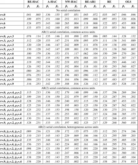
Tables 1-4 present Monte Carlo experiment results where each table corresponds to a
particular {𝑛,𝑇} combination. In particular, reported are the empirical probabilities of rejecting
the null hypotheses 𝛽1= 0.5 and 𝛽2= 5 (consistent with the DGP) based on t-tests. 5% critical
values were used so that the nominal level is 0.05. Thus, rejection probabilities that are close to
0.05 suggest that the test has the correct size, whereas probabilities above (below) 0.05 suggest
over-rejection (under-rejection) under the null hypothesis. The coefficient estimators performed
well under all scenarios, and common statistics corresponding with the coefficient estimators
(e.g. bias, efficiency, mean-squared error) are omitted for brevity.11 Several interesting patterns
emerge with respect to the three HAC covariance estimators. First, as conjectured above,
hypothesis tests using NW-HAC are severely distorted – in many cases by a factor of 5 or higher
– in the presence of unit effects (i.e. 𝑟 > 0) for all considered sample sizes. The rejection rates
have a similar pattern to those involving the usual OLS standard errors, which are of course
biased in the presence of a unit-specific effect. In particular, the null hypothesis with respect to
rate for relatively moderate (𝑟 = 0.6) or large (𝑟 = 0.9) between-unit variation. Performance
under both random effects and serial correlation reveals a similar pattern.
The new RE-HAC standard errors are an improvement over NW-HAC, although there
are size distortions evident in some simulations.
[Table 1 Here]
For 𝑛 = 5, 𝑇= 20, rejection rates for 𝛽1 are about 2.5 times too large – on average – across
scenarios. This size distortion increases with 𝑟. For 𝛽2, the tendency to over-reject the null
remains, but is less severe for the no serial correlation DGP. For the serial correlation DGPs, the
size distortion of 𝛽2 increases as the degree of serial correlation increases. Across these settings,
the average size is about 0.15 or 3 times the significance level. The size of the test statistics
improve with increases in 𝑛 and/or 𝑇. With 𝑛= 30, rejection rates for 𝛽1 have approximately the
correct size.
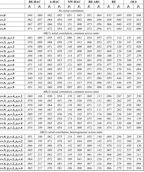
[Table 2 Here]
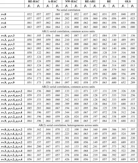
Although there is improvement, the tendency to over-reject the null for 𝛽2 remains. Even with 𝑛
= 30 and 𝑇 = 50, the rejection rates for 𝛽2 are about 2.5 times too large for moderate values of 𝑟
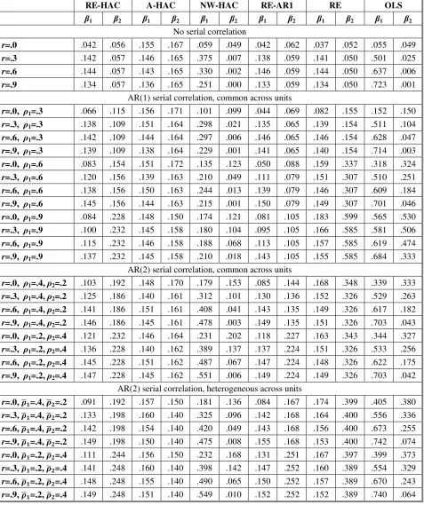
and a moderate degree of serial correlation. RE-HAC in particular performs poorly under the
AR(2) specification, especially with 𝜌2= 0.4, and this is presumably due to the use of the
AR(1)-based bandwidth selection procedure. Overall, for 𝛽1, the RE-HAC rejection rates are similar to
tests based on RE-AR1. For 𝛽2, however, RE-AR1 performs much better when the DGP is
random effects with AR(1) serial correlation – which is to be expected since the estimator is fully
consistent with the DGP; but, the performance of the two estimators is comparable under AR(2)
The size of tests based on A-HAC is rather promising. For each {𝑛,𝑇} combination,
there is very little variation in the rejection rates across the DGPs. For 𝑛 = 5, rejection rates are
approximately 3 times too high. For 𝑛 = 30, however, tests have approximately the correct size:
about 0.06 or 6%. There is no evidence of improvement with respect to an increase in 𝑇.
[Tables 3 and 4 Here]
One interesting observation is that for 𝑛 = 30 and the AR(1) DGP, the size of A-HAC tests is
closer to the nominal 5% level than for RE-AR1. In other words, even though RE-AR1 is fully
consistent with the DGP, A-HAC is more accurate for this sample size. In comparison to
RE-HAC, A-HAC rejection rates are closer to the nominal level for the serial correlation DGPs for 𝑛
= 30, and for 𝑛 = 5 with high degrees of serial correlation. RE-HAC rejection rates are closer to
the nominal level for 𝑛 = 5 for the no serial correlation DGP and the AR(1) DGP with a low or
moderate degree of serial correlation.
5. Further Explorations
The results from the Monte Carlo experiment motivate some further explorations. First,
the lack of size variation across DGPs for A-HAC, and its improvement for an increase in 𝑛,
suggests that a degrees of freedom correction, based on 𝑛, is justified. In fact, Stata and Limdep
both estimate 𝐕𝑖 using 𝑛
𝑛−1𝐕�𝑖𝐴−𝐻𝐴𝐶. For 𝑛 = 5, the size of A-HAC tests using this degrees of
freedom adjustment improves from about 0.15 to 0.12. For 𝑛 = 30 the improvement is from
about 0.06 to 0.055. Thus, the degrees of freedom correction appears desirable although for small
𝑛 the size distortion remains. This same degrees of freedom adjustment does not appear justified
for RE-HAC, as size improves for an increase in 𝑇 as well as 𝑛 and under no serial correlation
Second, the superior performance of A-HAC over RE-HAC for 𝑛 = 30 begs the question
of whether it is desirable to set bandwidth equal to 𝑇 rather than use a bandwidth selection
method. To gain some insight, several RE-HAC simulations were conducted where bandwidth
was simply set equal to 𝑇. The result was that RE-HAC rejection rates are approximately equal
to A-HAC. For example, with 𝑛 = 5, 𝑇 = 50, r = .6 and 𝜌1= 0.6, the rejection rate is .143 for 𝛽1
and .163 for 𝛽2. For the same sample size, but with r = .9, 𝜌̅1= 0.2 and 𝜌̅2= 0.4 the rates are .149
and .157, respectively. Similar results are obtained for the other three {𝑛, 𝑇} combinations.
Third, given the relative performance of RE-HAC over A-HAC with 𝑛 = 5 and low to
moderate AR(1) serial correlation, I explored the effect of using a prewhitening filter. Using the
VAR(1) prewhitening procedure proposed by Andrews and Monahan (1992), I find that test
statistics are much closer to the correct size for 𝑇 = 20 and 𝑇 = 50. In particular, even for 𝜌1=
0.9, the rejection rates for the AR(1) DGP approximate those from the analogous no serial
correlation DGP. In other words, there is no additional distortion from the serial correlation and
what is left is the distortion due to the random effect (which is also present for the RE and
RE-AR1 estimators). One caveat, however, is that the prewhitening helps very little for the case of
AR(2) serial correlation. What is happening is that the filter essentially removes all the
first-order serial correlation and the bandwidth selection procedure, based on an AR(1) serial
correlation model, leads to a bandwidth choice that is too small. The small bandwidth fails to
capture the second-order serial correlation. When a higher-order process is suspected, the
bandwidth selection procedure of Newey and West (1994) is likely preferable, as it is not based
6. Recommendations
Experimentalists analyzing panel data, like any analysts, should initially examine their
data to discern important properties. One can look at the time-series properties of the data by
usual time-series methods. For example, plotting the data against time can be used to examine
for trends. And, one can gain insight as to the type of autoregressive and/or moving average
process at play by examining the partial autocorrelation function and the autocorrelation
function. Wooldridge (2002) proposes a test of AR(1) serial correlation for panel data, which
requires minimal assumptions.12 There are a number of proposed approaches for unit-root
testing, and a review of this literature is provided by Baltagi and Kao (2000). If serial correlation
is a concern, which is likely for data from repeated-game experiments, this study provides some
recommendations on how to proceed using HAC covariance estimators for panel data.
So what is the bottom line? When there is a moderate (or large) number of cross-section
units per treatment, which is normal for experiments when data are at the participant-level, the
Monte Carlo results suggest that A-HAC (a.k.a. the “cluster-robust” covariance estimator) or the
covariance estimator proposed in this study (RE-HAC) with bandwidth equal to 𝑇are desirable
covariance estimators for OLS when there are unobserved unit effects and/or serial correlation of
unknown form.13,14 Hypothesis tests based these HAC covariance estimators have approximately
the correct size. As such, the HAC covariance estimators are as accurate as the RE or RE-AR1
estimator, even when one of the latter estimators are fully consistent with the DGP. When the
structure of the serial correlation is misspecified, RE-AR1 or related estimators will lead to
biased tests, and A-HAC will be preferred in such instances. Evidence from previous Monte
Carlo studies (Bertrand, Duflo, and Mullainathan 2004; Kezdi 2004) provides additional support
On the other hand, if the number of cross-section units per treatment is small, which is
more likely when data are at the group-level, such as a case where the experimentalist wishes to
analyze measures of market or social efficiency, recommendations are less clear. A-HAC (or
RE-HAC with bandwidth equal to 𝑇) standard errors tend to be too small. RE-HAC in tandem
with a prewhitening filter and data-dependent bandwidth selection appears to have promise, but
additional research is warranted. Certainly an analyst who is uncertain about the underlying DGP
should look to the RE-HAC estimator, rather than assume a particular structure for the serial
correlation as there may be greater size distortion due to misspecification. And it is noted that
estimators like RE-AR1 that place structure on the serial correlation, even if approximately
correctly specified, produce biased test statistics in small samples (see, for example, Table 1).
On a final note, the HAC covariance estimators investigated are generalizations of the
oft-used White’s (1980) heteroskedasticity-consistent covariance estimator. As such, although
the Monte Carlo simulations here do not consider DGPs with conditional heteroskedasticity,
A-HAC and RE-A-HAC are likewise robust to conditional heteroskedasticity of unknown form. In
fact, conditional heteroskedasticity is unlikely to cause any additional size distortions. Evidence
in support of these claims for A-HAC can be found in Bertrand, Duflo, and Mullainathan (2004)
and Kezdi (2004).
References
Andrews, Donald W. K. 1991. Heteroskedasticity and Autocorrelation Consistent Covariance
Matrix Estimation. Econometrica 59: 817-854.
Andrews, Donald W. K. and Christopher Monahan. 1992. An Improved Heteroskedasticity and
Autocorrelation Consistent Covariance Matrix Estimator. Econometrica 60: 953-966.
Arellano, M. 1987. Computing Robust Standard Errors for Within-Groups Estimators. Oxford
Bulletin of Economics and Statistics 49: 431-434.
Arellano, Manuel. 2003. Panel Data Econometrics. Oxford, UK: Oxford University Press.
Ashraf, Nava, Iris Bohnet, and Nikita Piankov. 2006. Decomposing Trust and Trustworthiness.
Experimental Economics 9: 193-208.
Ashley, R., S. Ball, and Catherine Eckel. 2003. Analysis of Public Goods Experiments Using
Dynamic Panel Regression Models. Working Paper, Department of Economics, Virginia
Tech.
Baker, Ronald J., James M. Walker, and Arlington W. Williams. 2009. Matching Contributions
and the Voluntary Provision of a Pure Public Good: Experimental Evidence. Journal of
Economic Behavior and Organization 70: 122-134.
Baltagi, Badi H. and Chihwa Kao. 2000. Nonstationary Panels, Cointegration in Panels and
Dynamic Panels: A Survey. Advances in Econometrics 15, 7-51.
Beck, N., and J.N. Katz. 1995. What to Do (and Not to Do) with Times-Series-Cross-Section
Data. American Political Science Review 89: 634-647.
Bertrand, Marianne, Ester Duflo, and Sendhil Mullainathan. 2004. How Much Should We Trust
Cushing, Matthew J. and Mary G. McGarvey. 1999. Covariance Matrix Estimation, in
Generalized Method of Moments Estimation, L. Matyas (ed.). New York: Cambridge
University Press.
Davis, Douglas D. and Charles A. Holt. 1993. Experimental Economics. Princeton, New Jersey:
Princeton University Press.
den Haan, Wouter J. and Andrew Levin. 1997. A Practitioner’s Guide to Robust Covariance
Matrix Estimation, in Handbook of Statistics 15, G. S. Maddala and C. R. Rao (eds.).
Amsterdam: Elsevier.
Driscoll, John C. and Aart C. Kraay. 1998. Consistent Covariance Matrix Estimation with
Spatially Dependent Panel Data. Review of Economics and Statistics 80: 549-560.
Drukker, David M. 2003. Testing for Serial Correlation in Linear Panel-Data Models. The Stata
Journal 3: 168–177.
Flood, Robert P. and Andrew K. Rose. 2002. Uncovered Interest Parity in Crisis. IMF Staff
Papers 49: 252-266.
Greene, William H. 2002. Econometric Analysis, 5th edition. Upper Saddle River, N.J.: Prentice
Hall.
Keifer, Nicholas M. and Timothy J. Vogelsang. 2002. Heteroskedasticity –Autocorrelation
Robust Testing Using Bandwidth Equal to Sample Size. Econometric Theory 18:
1350-1366.
Keifer, Nicholas M. and Timothy J. Vogelsang. 2005. A New Asymptotic Theory for
Heteroskedasticity-Autocorrelation Robust Tests. Econometric Theory 21: 1130-1164.
Kezdi, Gabor. 2004. Robust Standard Errors Estimation in Fixed-Effects Panel Models.
Newey, Whitney K. and Kenneth D. West. 1987. A Simple, Positive Semi-Definite,
Heteroscedasticity and Autocorrelation Consistent Covariance Matrix. Econometrica 55:
703-708.
Newey, Whitney K. and Kenneth D. West. 1994. Automatic Lag Selection in Covariance
Estimation. Review of Economic Studies 61: 631-654.
Rassenti, S.J., V.L. Smith, and B.J. Wilson. 2003. Controlling Market Power and Price Spikes in
Electricity Networks: Demand-Side Bidding. Proceedings of the National Academy of
Sciences 100: 2998-3003.
Shupp, Robert S. and Arlington W. Williams. 2008. Risk Preference Differentials of Small
Groups and Individuals. Economic Journal 118: 258-283.
White, Hal. 1980. A Heteroskedasticity-Consistent Covariance Matrix Estimator and a Direct
Test for Heteroskedasticity. Econometrica 40: 617-636.
White, Hal. 1982. Maximum Likelihood Estimation of Misspecified Models. Econometrica 50:
1-25.
White, Hal. 1984. Asymptotic Theory for Econometricians. Orlando, FL: Academic Press.
Wooldridge, Jeffrey M. 2002. Econometric Analysis of Cross Section and Panel Data.
Table 1. Monte Carlo Results: Null Rejection Probabilities for 𝒏 = 5,𝑻 = 20
RE-HAC A-HAC NW-HAC RE-AR1 RE OLS
β1 β2 β1 β2 β1 β2 β1 β2 β1 β2 β1 β2
No serial correlation
r=.0 .041 .065 .136 .155 .057 .051 .045 .072 .035 .047 .046 .046 r=.3 .109 .075 .151 .160 .252 .013 .099 .068 .097 .053 .320 .026 r=.6 .124 .075 .143 .160 .265 .004 .118 .068 .122 .053 .453 .008 r=.9 .133 .075 .142 .160 .192 .000 .135 .068 .133 .053 .561 .001
AR(1) serial correlation, common across units
r=.0, ρ1=.3 .078 .114 .135 .146 .101 .090 .055 .086 .085 .144 .128 .132
r=.3, ρ1=.3 .112 .120 .153 .147 .231 .038 .095 .079 .111 .138 .341 .089
r=.6, ρ1=.3 .120 .120 .146 .147 .242 .009 .111 .078 .119 .138 .450 .043
r=.9, ρ1=.3 .130 .120 .142 .147 .189 .001 .130 .078 .131 .138 .560 .007
r=.0, ρ1=.6 .100 .179 .136 .153 .151 .117 .062 .104 .150 .299 .270 .261
r=.3, ρ1=.6 .104 .192 .135 .152 .199 .076 .084 .101 .121 .293 .387 .217
r=.6, ρ1=.6 .119 .192 .144 .152 .219 .032 .105 .101 .137 .293 .446 .143
r=.9, ρ1=.6 .126 .192 .134 .152 .192 .004 .118 .101 .130 .293 .560 .027
r=.0, ρ1=.9 .080 .261 .135 .175 .176 .103 .096 .135 .107 .492 .415 .351
r=.3, ρ1=.9 .076 .253 .142 .159 .196 .083 .090 .112 .115 .483 .444 .329
r=.6, ρ1=.9 ..086 .253 .134 .159 .184 .056 .096 .112 .107 .483 .457 .277
r=.9, ρ1=.9 .116 .253 .142 ,159 .188 .016 .126 .112 .131 .483 .528 .141
AR(2) serial correlation, common across units
r=.0, ρ1=.4, ρ2=.2 .115 .213 .136 .152 .179 .140 .099 .146 .137 .296 .269 .264
r=.3, ρ1=.4, ρ2=.2 .109 .218 .134 .150 .232 .079 .097 .150 .123 .287 .391 .202
r=.6, ρ1=.4, ρ2=.2 .128 .218 .146 .150 .240 .032 .115 .150 .134 .287 .453 .131
r=.9, ρ1=.4, ρ2=.2 .125 .218 .135 .150 .195 .003 .125 .150 .128 .287 .562 .022
r=.0, ρ1=.2, ρ2=.4 .125 .232 .135 .153 .198 .158 .120 .206 .130 .275 .251 .231
r=.3, ρ1=.2, ρ2=.4 .121 .231 .137 .151 .253 .083 .109 .217 .124 .268 .385 .173
r=.6, ρ1=.2, ρ2=.4 .130 .231 .144 .151 .255 .032 .123 .217 .132 .268 .455 .107
r=.9, ρ1=.2, ρ2=.4 .128 .231 .133 .151 .197 .002 .125 .217 .129 .268 .560 .018
AR(2) serial correlation, heterogeneous across units
Table 2. Monte Carlo Results: Null Rejection Probabilities for 𝒏 = 30,𝑻 = 20
RE-HAC A-HAC NW-HAC RE-AR1 RE OLS
β1 β2 β1 β2 β1 β2 β1 β2 β1 β2 β1 β2
No serial correlation
r=.0 .044 .060 .062 .065 .051 .045 .051 .064 .033 .049 .050 .048 r=.3 .062 .057 .064 .054 .195 .002 .060 .056 .058 .040 .319 .013 r=.6 .067 .057 .066 .054 .151 .000 .073 .056 .066 .040 .435 .002 r=.9 .071 .057 .072 .054 .102 .000 .072 .056 .071 .040 .522 .000
AR(1) serial correlation, common across units
r=.0, ρ1=.3 .063 .089 .055 .052 .086 .061 .034 .053 .074 .112 .131 .103
r=.3, ρ1=.3 .070 .089 .068 .059 .178 .012 .066 .052 .072 .120 .347 .058
r=.6, ρ1=.3 .076 .089 .071 .059 .149 .000 .069 .052 .078 .120 .472 .020
r=.9, ρ1=.3 .068 .089 .072 .059 .110 .000 .069 .052 .069 .120 .548 .000
r=.0, ρ1=.6 .056 .146 .053 .053 .114 .077 .053 .080 .100 .271 .257 .239
r=.3, ρ1=.6 .066 .142 .062 .053 .132 .024 .061 .078 .089 .270 .388 .175
r=.6, ρ1=.6 .071 .142 .065 .053 .121 .005 .069 .078 .077 .270 .460 .090
r=.9, ρ1=.6 .073 .142 .069 .053 .113 .000 .071 .078 .076 .270 .541 .004
r=.0, ρ1=.9 .036 .154 .068 .057 .115 .035 .064 .083 .054 .439 .396 .291
r=.3, ρ1=.9 .040 .162 .065 .050 .107 .031 .071 .088 .059 .446 .395 .261
r=.6, ρ1=.9 .039 .162 .062 .050 .111 .017 .070 .088 .053 .446 .439 .209
r=.9, ρ1=.9 .051 .162 .060 .050 .095 .001 .058 .088 .058 .446 .497 .057
AR(2) serial correlation, common across units
r=.0, ρ1=.4, ρ2=.2 .060 .168 .050 .054 .139 .087 .069 .113 .094 .267 .267 .230
r=.3, ρ1=.4, ρ2=.2 .070 .160 .062 .051 .156 .026 .070 .111 .083 .262 .397 .156
r=.6, ρ1=.4, ρ2=.2 .070 .160 .064 .051 .139 .003 .071 .111 .077 .262 .470 .081
r=.9, ρ1=.4, ρ2=.2 .074 .160 .067 .051 .116 .000 .072 .111 .077 .262 .550 .002
r=.0, ρ1=.2, ρ2=.4 .069 .197 .053 .056 .156 .102 .072 .176 .080 .236 .249 .202
r=.3, ρ1=.2, ρ2=.4 .072 .189 .065 .054 .174 .026 .075 .168 .081 .230 .391 .139
r=.6, ρ1=.2, ρ2=.4 .073 .189 .065 .054 .156 .003 .075 .168 .074 .230 .468 .065
r=.9, ρ1=.2, ρ2=.4 .074 .189 .068 .054 .118 .000 .072 .168 .074 .230 .547 .000
AR(2) serial correlation, heterogeneous across units
Table 3. Monte Carlo Results: Null Rejection Probabilities for 𝒏 = 5,𝑻 = 50
RE-HAC A-HAC NW-HAC RE-AR1 RE OLS
β1 β2 β1 β2 β1 β2 β1 β2 β1 β2 β1 β2
No serial correlation
r=.0 .042 .056 .155 .167 .059 .049 .042 .062 .037 .052 .055 .049 r=.3 .142 .057 .146 .165 .375 .007 .138 .059 .141 .050 .501 .025 r=.6 .144 .057 .143 .165 .330 .002 .146 .059 .144 .050 .637 .006 r=.9 .134 .057 .136 .165 .251 .000 .133 .059 .134 .050 .723 .001
AR(1) serial correlation, common across units
r=.0, ρ1=.3 .066 .115 .156 .171 .101 .099 .044 .069 .082 .155 .152 .150
r=.3, ρ1=.3 .138 .109 .151 .164 .298 .021 .135 .065 .139 .154 .511 .104
r=.6, ρ1=.3 .142 .109 .144 .164 .297 .006 .146 .065 .146 .154 .628 .047
r=.9, ρ1=.3 .139 .109 .138 .164 .229 .001 .141 .065 .140 .154 .714 .003
r=.0, ρ1=.6 .083 .154 .151 .172 .135 .123 .050 .088 .159 .337 .318 .324
r=.3, ρ1=.6 .120 .156 .139 .163 .210 .049 .111 .079 .151 .307 .510 .251
r=.6, ρ1=.6 .138 .156 .150 .163 .244 .013 .139 .079 .146 .307 .609 .184
r=.9, ρ1=.6 .145 .156 .144 .163 .215 .001 .150 .079 .149 .307 .701 .046
r=.0, ρ1=.9 .084 .228 .148 .150 .174 .121 .081 .105 .183 .599 .565 .530
r=.3, ρ1=.9 .100 .232 .145 .158 .180 .104 .095 .105 .166 .585 .581 .506
r=.6, ρ1=.9 .115 .232 .146 .158 .188 .068 .113 .105 .157 .585 .619 .474
r=.9, ρ1=.9 .137 .232 .145 .158 .210 .018 .143 .105 .155 .585 .684 .333
AR(2) serial correlation, common across units
r=.0, ρ1=.4, ρ2=.2 .103 .192 .148 .170 .179 .153 .085 .144 .168 .348 .339 .333
r=.3, ρ1=.4, ρ2=.2 .125 .186 .140 .161 .312 .101 .130 .136 .152 .326 .529 .263
r=.6, ρ1=.4, ρ2=.2 .141 .186 .151 .161 .408 .041 .143 .135 .149 .326 .617 .182
r=.9, ρ1=.4, ρ2=.2 .146 .186 .145 .161 .478 .003 .149 .135 .151 .326 .703 .043
r=.0, ρ1=.2, ρ2=.4 .121 .232 .146 .164 .231 .202 .118 .227 .163 .343 .344 .327
r=.3, ρ1=.2, ρ2=.4 .136 .228 .140 .162 .389 .137 .137 .224 .151 .326 .533 .256
r=.6, ρ1=.2, ρ2=.4 .145 .228 .151 .162 .487 .067 .147 .224 .148 .326 .622 .175
r=.9, ρ1=.2, ρ2=.4 .147 .228 .145 .162 .551 .006 .149 .224 .149 .326 .703 .042
AR(2) serial correlation, heterogeneous across units
Table 4. Monte Carlo Results: Null Rejection Probabilities for 𝒏 = 30,𝑻 = 50
RE-HAC A-HAC NW-HAC RE-AR1 RE OLS
β1 β2 β1 β2 β1 β2 β1 β2 β1 β2 β1 β2
No serial correlation
r=.0 .032 .057 .057 .069 .050 .052 .037 .062 .031 .055 .048 .055 r=.3 .057 .057 .057 .064 .282 .002 .058 .060 .056 .056 .499 .023 r=.6 .061 .057 .062 .064 .213 .000 .062 .060 .061 .056 .633 .006 r=.9 .063 .057 .064 .064 .124 .000 .063 .060 .063 .056 .696 .000
AR(1) serial correlation, common across units
r=.0, ρ1=.3 .061 .105 .056 .066 .092 .087 .037 .072 .084 .159 .139 .156
r=.3, ρ1=.3 .058 .095 .059 .064 .210 .010 .057 .063 .062 .140 .489 .091
r=.6, ρ1=.3 .061 .095 .062 .064 .182 .000 .060 .063 .062 .140 .619 .027
r=.9, ρ1=.3 .063 .095 .063 .064 .124 .000 .059 .063 .063 .140 .696 .000
r=.0, ρ1=.6 .058 .122 .061 .068 .103 .095 .043 .084 .128 .319 .316 .308
r=.3, ρ1=.6 .053 .124 .055 .060 .150 .019 .056 .072 .074 .314 .498 .250
r=.6, ρ1=.6 .055 .124 .059 .060 .144 .001 .056 .072 .063 .314 .598 .156
r=.9, ρ1=.6 .063 .124 .062 .060 .102 .000 .063 .072 .064 .314 .685 .013
r=.0, ρ1=.9 .048 .163 .067 .060 .099 .077 .056 .072 .100 .579 .565 .502
r=.3, ρ1=.9 .046 .173 .060 .064 .123 .069 .058 .079 .082 .600 .556 .499
r=.6, ρ1=.9 .054 .173 .061 .064 .117 .034 .055 .079 .076 .600 .581 .456
r=.9, ρ1=.9 .051 .173 .058 .064 .097 .002 .058 .079 .063 .600 .652 .289
AR(2) serial correlation, common across units
r=.0, ρ1=.4, ρ2=.2 .064 .156 .060 .069 .133 .121 .071 .137 .131 .339 .326 .320
r=.3, ρ1=.4, ρ2=.2 .059 .153 .055 .060 .251 .060 .059 .128 .073 .333 .510 .256
r=.6, ρ1=.4, ρ2=.2 .059 .153 .060 .060 .342 .013 .058 .128 .062 .333 .609 .157
r=.9, ρ1=.4, ρ2=.2 .064 .153 .063 .060 .389 .000 .065 .128 .064 .333 .688 .013
r=.0, ρ1=.2, ρ2=.4 .085 .203 .060 .067 .194 .163 .095 .204 .125 .339 .336 .324
r=.3, ρ1=.2, ρ2=.4 .061 .196 .057 .059 .344 .105 .067 .197 .072 .338 .512 .246
r=.6, ρ1=.2, ρ2=.4 .061 .196 .060 .059 .426 .024 .058 .197 .062 .338 .609 .151
r=.9, ρ1=.2, ρ2=.4 .064 .196 .064 .059 .483 .000 .065 .197 .064 .338 .688 .012
AR(2) serial correlation, heterogeneous across units
1
Note that the idea for this paper originated in 2002, when panel data analysis was the exception rather than the rule
for drawing inferences from experimental data. Although panel data models are increasing used for analyzing
repeated-game experiment data, and indeed more and more researchers have relied on using cluster-robust standard
errors, it remains common for journal referees to request simple statistical tests even when their validity is
questionable.
2
Indeed, on numerous occasions I have reviewed papers that simply mention heteroskedasticity when justifying the
use of cluster-robust standard errors. Further, it is fairly common for some to use the standard random effects
estimator in tandem with cluster-robust standard errors. This approach is internally inconsistent, as the random
effects estimator assumes a specific form of within-unit serial correlation but the use of cluster-robust standard
errors suggests that the assumed form of serial correlation is incorrect.
3
Data sets of this sort tend to be labeled as “time-series cross-section” or TSCS data.
4
A prewhitening filter attempts to remove some correlation in the residuals from a regression model, which has
been shown to improve the performance of HAC-based techniques (see Andrews and Monahan 1992).
5
Stata’s newey command (with option force) produces standard OLS coefficients (without any adjustment for a
fixed or random-effects structure) along with the NW-HAC estimator. Limdep estimates an equivalent NW-HAC
estimator, but with a fixed-effects estimator for model coefficients.
6
This covariance estimator is produced when one specifies the cluster option for Stata or Limdep’s regress
command. To estimate a fixed-effects model with A-HAC errors in Stata, one can jointly use the cluster and fe
options for Stata’s xtreg command.
7
For purpose of identification, the HAC covariance estimators considered here require that 𝑛 ≥ 𝑘.
8
Of course, this estimator would be inefficient, and the standard FGLS random effects estimator for β is preferable.
9
As suggested by Andrews (1991), to calculate the bandwidths I use a weight of 0 for the autoregressive parameter
associated with the model intercept and a weight of 1 on other autoregressive parameters. See Andrews (1991) for
details on using this procedure.
10
OLS and random effects models are estimated using canned procedures in Limdep. RE-AR1 uses an estimate of ρ
from a fixed effects model. To construct the RE-HAC covariance estimator I use the estimate of 𝜎𝑢2 generated by
Limdep’s random effects estimator.
11
12
There is a user-written program available to run this test in Stata (Drukker, 2003).
13
Since there are canned procedures in Stata and Limdep for A-HAC (with the degrees of freedom correction
discussed above), it is likely preferable from the practitioner’s viewpoint.
14
If a fixed-effects structure is preferred or assumed, then a fixed effects coefficient estimator with A-HAC is