Line Graphs and Quasi-total Graphs
Bhavanari Satyanarayana
Department of Mathematics, Acharya Nagarjuna University,Nagarjuna Nagar – 522 510, A. P., India.
Devanaboina Srinivasulu
Department of Mathematics, Acharya Nagarjuna University,Nagarjuna Nagar – 522 510, A. P., India.
Kuncham Syam Prasad
Department of Mathematics, Manipal Institute of Technology,Manipal University, Manipal – 576 104, India,
ABSTRACT
The line graph, 1-quasitotal graph and 2-quasitotal graph are well-known. It is proved that if G is a graph consist of exactly m connected components Gi, 1 i m, then L(G) = L(G1)
L(G2) … L(Gm) where L(G) denotes the line graph of G,
and „‟ denotes the ring sum operation on graphs. The number of connected components in G is equal to the number of connected components in L(G) and also if G is a cycle of length n, then L(G) is also a cycle of length n. The concept of 1-quasitotal graph is introduced and obtained that Q1(G) = G
L(G) where Q1(G) denotes 1-quasitotal graph of a given
graph G. It is also proved that for a 2-quasitotal graph of G, the two conditions (i) |E(G)|= 1; and (ii) Q2(G) contains
unique triangle are equivalent.
General Terms
Graph Theory, line graphs, ring sum operation on graphs.
Keywords
Line graph, quasi total graph, connected component.
1.
LINE GRAPHS
All graphs considered are finite and simple. For standard literature on graph theory we refer Bondy and Murty [1], Harary [2], Satyanarayana and Syam Prasad [7, 8].
We start this section with the following remark.
1.1 Remark: Let G be a graph with E(G)
, and L(G) its line graph.(i) V(G)
V(L(G)) =
.(ii) E(G)
E(L(G)) =
.1.2 Lemma: Let G be a graph. Suppose G1, G2 are two
connected components of a graph G. Write G = G1
G2.Suppose e1, e2
G such that s = e e12 E(L(G)).
If e1
E(G1), then e2 E(G
1) but not e2
E(G2) (In otherwords, if s1
E(G
1) and s2 E(G
2), then s1 and s2 cannot beadjacent in L(G)).
Proof: Suppose e1 G1. Since e2 E(G) = E(G1) E(G2),
either e2 E(G1) or e2 E(G2). Now to show that
e2 E(G2). If possible, suppose that e2 E(G2).
Since s = e e1 2 E(L(G)), we have that e1 is adjacent to e2.
Then e1 = v v1 2 and e2 = v v2 3 for some v1, v2, v3 V(G).
Since e1 E(G1) and e2 E(G2), we have that v1, v2 V(G1),
v2, v3 V(G2). So v2 V(G1) V(G2).
Take x, y G1 G2. If x, y G1 (or G2), then since G1 (or
G2) is a connected component, we have that there is a path
from x to y. Suppose x G1 and y G2.
Since x, v2 G1, there is a path from x to v2; and since v2,
y G2 there is a path from v2 to y in G2. These paths
combined together must provide a path from x to y. This shows that G1 G2 is connected, a contradiction to the fact
that G1 and G2 are two different connected components of a
graph. Hence e2 E(G2) and e2 E(G1).
1.3 Lemma: If G = G1
G2 where G1 and G2 are twoconnected graphs with V(G1)
V(G2) =
, then L(G) =L(G1)
L(G2).Proof: Since G1
G, E(G1)
E(G).Also E(G2)
E(G). V(L(G1))
V(L(G2)) =E(G1)
E(G2) = E(G) = V(L(G)) … (i)Let s E(L(G1)). Then s = e e1 2where e1, e2
E(G1), ande1 and e2 are adjacent in G1
s = e e1 2 and e1, e2 E(G1)
E(G), and e1, e2 are adjacent in G1
G.
s E(L(G)). Therefore E(L(G1))
E(L(G)).In a similar way we get E(L(G2))
E(L(G)).So L(G1)
L(G2)
L(G) …(ii)Let s
E(L(G)). Then s =
e e1 2 for some e1, e2 V(L(G))
= E(G), and e1, e2 are adjacent in G.
By Lemma 1.2, e1, e2
E(G
1) or e1, e2
E(G2), but notboth. If e1, e2
E(G
1), then since e1, e2 are adjacent in G, e1,e2 are adjacent in G1 and so s = e e1 2
E(L(G
1)).Similarly, if e1, e2 E(G2), then s = e e1 2 E(L(G2)).
Hence E(L(G))
E(L(G1))
E(L(G2)) … (iii)From (ii) and (iii), E(L(G)) = E(L(G1))
E(L(G2)) … (iv)Since G = G1
G2, it follows that E(G1)
E(G2) =
.Now from (i) and (iv), L(G) = L(G1)
L(G2), the proof iscomplete.
1.4 Example: Consider the graphs G1 and G2 given in Fig. 1
Fig 1
Fig 2
The ring sum of G1 and G2 is given in Fig. 3
Fig 3
The line graph of G1 and G2 are given in Fig. 4 and Fig. 5
respectively.
Fig 4
Fig 5
The line graph L(G) is given in Fig. 6
Fig 6
Now let us construct the ring sum of L(G1) and L(G2).
V(L(G1) L(G2)) = {e1, e2, f1, f2, f3, f4}, and
E(L(G1) L(G2)) = {e e1 2, f f1 2, f f1 3, f f2 3, f f3 4, f f2 4}.
The graph L(G1) L(G2) is same as the graph given in Fig.6.
It is an easy observation that L(G) = L(G1) L(G2).
1.5 Theorem: If G is a graph consists of exactly m connected components G1, G2, …, Gm, then L(G) = L(G1) L(G2) …
L(Gm).
Proof: The proof is by induction on m.
If m = 2, then it follows through the above Lemma 1.3. Suppose that the result is true for m = k.
Now take a graph G with m = k + 1 connected components G1, G2, …, Gk+1.
Now G = G1 G2 … Gk Gk+1 = (G1 G2 … Gk)
Gk+1.
Now L(G) = L((G1 G2 … Gk) (Gk+1))
= L(G1 G2 … Gk) + L(Gk+1) (by Lemma 1.3)
= L(G1) L(G2) … L(Gk) L(Gk+1) (by
induction hypothesis), the proof is complete.
1.6 Lemma: If G is a connected graph, then L(G) is also a connected graph.
Proof: Let G be a connected graph. To show that L(G) is connected, let e1, e2 V(L(G)) = E(G).
Suppose e1 = uv and e2 = xy for some u, v, x, y V(G).
Since G is connected, there exists a path from v to x. Suppose this path is vf1v1f2v2 …fkvk with vk = x.
Since f1 is adjacent to f2, f2 is adjacent to f3, … fk-1 is adjacent
to fk, it follows that f f1 2, f f2 3, … f fk-1 k is a path from f1 to fk
in L(G).
If e1 = f1 and fk = e2, then f f1 2, f f2 3, …, f fk-1 k is a path from
e1 to e2 in L(G).
If e1 f1 and fk = e2, then e f1 1,f f1 2, f f2 3, …, f fk-1 k is a path from e1 to e2 in L(G).
If e1 f1 and fk e2, then e f1 1, f f1 2, ..., f fk-1 k, f ek 2 is a path from e1 to e2 in L(G).
If e1 = f1 and fk e2, then f f1 2, f f2 3, …, f fk-1 k, f ek 2 is a path
from e1 to e2 in L(G).
Hence for any e1, e2 V(L(G)), there is a path between e1 &
e2 in L(G). This shows that L(G) is connected, the proof is
complete.
1.7 Theorem: The number of connected components in G is equal to the number of connected components in L(G).
Proof: Suppose the connected components of G are G1, G2,
…, Gk.
Then G = G1 G2 … Gk.
By Theorem 1.6, L(G) = L(G1) L(G2) … L(Gk).
G
1e
1e
2
v3
v1
x
1
v2
G
2 x1f
4f3
f2
f
1x2
x3
x4G = G1 G2
e1
e2
v3
v1
x
1
v2
x1
f4
f3
f2
f
1x2
x3
x4e1
e2
L(G1):
f3
f2
f1
f4
L(G2):
e1
e2
f1 f2
f3
Since Gi is connected by Lemma1.6, the graph L(Gi) is
connected and so L(Gi) is a connected component of L(G).
Hence L(G) = L(G1) L(G2) … L(Gk) and each L(Gi)
is connected.
Thus the number of components of G = k = the number of components of L(G), the proof is complete.
1.8 Theorem: If G is a cycle of length n, then L(G) is also a cycle of length n.
Proof: Suppose G is a cycle of length n.
Then V(G) = {v1, v2, …, vn}, and E(G) = {e1, e2, …, en} with
the cycle v1e1v2e2…vnenv1.
Now V(L(G)) = E(G) = {e1, e2, …, en}.
Since ei-1 and ei for 2 i n are adjacent in G, we get that
i-1 i
e e L(G) for 2 i n. Since e1 and en have common
vertex v1 in G, we have that e e1 n L(G).
Thus e e1 2, e e2 3, …, e en-1 n, e en 1 E(L(G)). Since these are only edges in L(G) we get that E(L(G))
= {e e1 2, e e2 3, …, e en-1 n, e en 1}. Thus L(G) is a cycle of length n.
2.
1-QUASITOTAL GRAPHS
We start this section by introducing a new concept “1-quasitotal graph”.
2.1 Definition: Let G be a graph with vertex set V(G) and edge set E(G). The 1–quasitotal graph, (denoted by Q1(G))
of G is defined as follows:
The vertex set of Q1(G), that is V(Q1(G)) = V(G) E(G).
Two vertices x, y in V(Q1(G)) are adjacent if they satisfy one
of the following conditions:
(i). x, y are in V(G) and xy E(G).
(ii). x, y are in E(G) and x, y are incident in G.
2.2 Note: (i) G is a subgraph of Q1(G); and
(ii) Q1(G) is a subgraph of T(G).
2.3 Example: Consider the graph G given in Fig. 7. Let us construct the 1-quasitotal graph Q1(G) of the graph G.
Fig 7
Fig 8
V(Q1(G)) = {V(G) E(G)} = {v1, v2, v3, v4, e1, e2, e3, e4}
It is clear that E(G) E(Q1(G)).
So v v1 4, v v4 3, v v3 2, v v2 1 E(Q1(G)).
Since e1 and e2 are incident in G, there is an edge e e1 2
E(Q1(G)). Since e1 and e4 are incident in G, there is an edge
1 4
e e E(Q1(G)). Since e2 and e3 are incident in G, there is
an edge e e2 3 E(Q1(G)). Since e3 and e4 are incident in G,
there is an edge e e3 4 E(Q1(G)). Therefore E(Q1(G)) =
{v v1 4,
v v
4 3, v v3 2, v v2 1, e e1 2, e e1 4, e e2 3, e e3 4}. The 1-quasitotal graph Q1(G) is given by the Fig. 8.2.4 Theorem: Q1(G) = G L(G).
Proof: By the definition of Q1(G),
V(Q1(G)) = V(G) E(G) = V(G) V(L(G)) (since V(L(G))
= E(G)). Let s E(G). If s is an edge in G, then s E(G). If s E(G), then (by the definition of Q1(G)) s = e e1 2 where
e1, e2 E(G) and e1, e2 are adjacent edges in G. By the
definition of L(G) it follows that s E(L(G)).
Therefore E(Q1(G)) E(G) E(L(G)). By Note 2.2, E(G)
E(L(G)) E(Q1(G)). Hence Q1(G) = G L(G), the union of
the two graphs G and L(G). Since V(G) V(L(G)) = V(G) E(G) = , there exists no common edge in G and L(G). This means that E(G) E(L(G)) = . This implies that G L(G) = G L(G).
Hence Q1(G) = G L(G) = G L(G), the proof is complete.
2.5 Corollary: If G is a cycle of length n, then Q1(G) is the
ring sum of exactly two disjoint cycles of length n.
Proof: Suppose G is a cycle of length n.
By Theorem1.8, L(G) is a cycle of length n.
Since Q1(G) = G L(G) (by Theorem 2.4) Q1(G) is equal to
the ring sum of two disjoint cycles of length n, the proof is complete.
3
. 2-QUASITOTAL GRAPHSWe start this section by introducing a new concept “2-quasitotal graph”.
3.1 Definition: Let G be a graph with vertex set V(G) and edge set E(G).
The 2-quasitotal graph of G, denoted by Q2(G) is defined as
follows: The vertex set of Q2(G), that is, V(Q2(G)) = V(G)
e4
e1
e2
e3
v1 v2
v4 v3
G
e4
e1
e2
e3
v1 v2
v4 v3
E(G). Two vertices x, y in V(Q2(G)) are adjacent in Q2(G) in
case one of the following holds:
(i) x, y are in V(G) and xy E(G).
(ii) x is in V(G); y is in E(G); and x, y are incident in G.
3.2 Note: (i) G is a subgraph of Q2(G); and
(ii) Q2(G) is a subgraph of T(G).
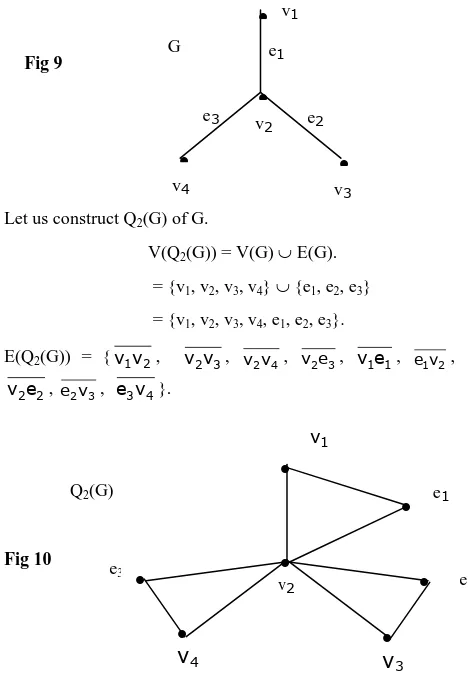
3.3 Example: Consider the graph given in fig 9.
Fig 9
Let us construct Q2(G) of G.
V(Q2(G)) = V(G) E(G).
= {v1, v2, v3, v4} {e1, e2, e3}
= {v1, v2, v3, v4, e1, e2, e3}.
E(Q2(G)) = {v v1 2, v v2 3, v v2 4, v e2 3, v e1 1, e v1 2,
2 2
[image:4.595.52.286.207.553.2]v e , e v2 3, e v3 4}.
Fig 10
The Q2(G) is given in Fig 10
3.4 Lemma: If e = uv
E(G), then there exist a triangle in E(Q2(G)) containing e as one of the edges.Proof: Suppose G is a graph with |E(G)| = 1. Let e E(G) and e = vu for some v, u V(G). Now e, v, u V(G) E(G) = V(Q2(G)).
Nowvu E(G) E(Q2(G)). Since e and u are incident in G,
we have that ue E(Q2(G)). Since e and v are incident in G,
we have that ev E(Q2(G)).
So vu, ue, ev E(Q2(G)) and these edges put together form
a triangle, the proof is complete.
3.5 Lemma: If e is not in a triangle of G and e = uv E(G) is
only the edge between the vertices u and v in G, then there is only one triangle in E(Q2(G)) containing e as one of the edges.
Proof: By Lemma 3.4, we know that uv, ve, eu is a triangle (in Q2(G)) containing the edge e = uv.
Let
ab
, bc, ca be a triangle in Q2(G) containing e = uv.Without loss of generality, we assume that ab = e and so ab
= uv. Further, we we assume that a = u and b = v.
If bc and ca are edges in G, then ab, bc, ca is a triangle in G containing e, a contradiction to our hypothesis. So bc or
ca is not in E(G).
Suppose bc is not in E(G). Since b V(G) it follows that c E(G).
Since bc is in E(Q2(G)), by the definitions of Q2(G), it
follows that the edge c of G is incident on the vertex b = v of G.
Now ca E(Q2(G)) implies that the edge c is incident on the
vertex a = u.
Thus c is an edge between its end points u and v.
Since there is only one edge (in G) between the vertices u and v, we get c = e.
Thus the triangle ab, bc, ca taken in E(Q2(G)) is nothing but
uv, ve, eu. Hence there is only one triangle in Q2(G)
containing (or corresponding to) e.
3.6 Note: If xy E(Q2(G)) \ E(G), then by the definition of
Q2(G) it follows that one of the x, y is edge (say x ) in G and
the edge x is incident on the vertex y (of G) in G.
3.7 Lemma: Every triangle in Q2(G) contains an edge of G.
Proof: Let ab, bc, ca be a triangle in Q2(G).
If possible suppose that neither ab nor bc nor ca is an edge in G.
Since ab is an edge in E(Q2(G)) \ E(G), one of the a, b is an
edge and the other is a vertex in G
Without loss of generality, assume that a E(G) and b V(G) and a is incident on b.
Since b V(G),
bc
E(Q2(G)) \ E(G), we have that c E(G) and c is incident on b.
Since ca E(Q2(G)) \ E(G) and c E(G), it follows that a
V(G) and c is incident on a. This fact a V(G) is a contradiction to the fact a E(G).
Thus one of the ab, bc, ca is an edge in G.
3.8 Theorem: If G is a graph containing only one edge (that is |E(G)| = 1) then the graph Q2(G) contains unique triangle.
Proof: (Existence): Let E(G) = {e} and u, v V(G) with
e = uv. By Lemma 3.4,
uv, ve, eu is a triangle in Q2(G) containing the edge e.
(Uniqueness): Since e is only the edge in G, the graph G contains no triangles. So the statement “e is not in any triangle of G” is true.
Thus by using Lemma 3.5, we can conclude that Q2(G)
contains only one triangle containing “e”… (i) e2
e3 v2
e1
v1
v3
v4 G
v2
v
4v
3v1
e2
e3
e1
Q2(G)
Now we verify that any triangle in Q2(G) contains e.
Let xy, yz, zx be a triangle in Q2(G).
By Lemma 3.7, this triangle contains an edge of G. Since G contains only one edge e, it follows that the triangle (xy, yz, zx) contains e. From the above steps, every triangle in Q2(G)
contains the edge “e” … (ii)
From (i) & (ii), we get that Q2(G) contains unique triangle.
3.9 Lemma: Suppose G contains two distinct edges e1 = uv
and e2 = xy (i) If {u, v} {x, y} =
, then Q2(G) containstwo distinct triangles one containing e1 and other containing
e2. Moreover there is no common vertex between two
triangles.
(ii) If {u, v} {x, y}
, then Q2(G) contains two distincttriangles one containing e1 and other containing e2.
Moreover if {a} = {u, v} {x, y}, then a is a common vertex to these two triangles.
Proof: Given that e1 = uv and e2 = xy are two edges in G.
By Lemma 3.4, ue1, e v1 , vu is a triangle in Q2(G)
containing e1 = uv; and
2
xe , e y2 , yx is a triangle in Q2(G) containing e2 = xy.
Clearly these are two distinct triangles.
Suppose that {u, v} {x, y} = .
If possible suppose that the triangles {ue1, e v1 , vu} and {xe2, e y2 , yx} have a common vertex.
The vertex sets of these triangles are {u, v, e1} and {x, y, e2}.
Since e1
e2 (as edges in G), e1
e2 (as vertices in Q2(G)).The remaining part is clear because {u, v} {x, y} = .
Hence there is no common vertex between the two triangles.
(ii)Suppose {u, v} {x, y}
. If {u, v} = {x, y}, then e1 = uv = xy = e2, a contradiction. So {u, v}
{x, y}, and {u,v} {x, y}
.Without loss of generality, assume that u = x and v y.
In this case, the vertex sets of the triangles are {u, v, e1} and
{x, y, e2} = {u, y, e2}.
This shows that the two triangles are having a common vertex u, the proof is complete.
3.10 Theorem: Let G be a graph. Then the following conditions are equivalent:
(i) |E(G)| = 1;
(ii) Q2(G) contains unique triangle.
Proof: (i) (ii): Theorem 3.8
(ii) (i): Suppose Q2(G) contains unique triangle. By
Lemma 3.7, every triangle of Q2(G) contains at least one edge
of G. Since Q2(G) contains a triangle, |E(G)| 1. If |E(G)| >
1, then E(G) contains two distinct edges. By Lemma 3.9, it follows that Q2(G) contains two distinct triangles, a
contradiction to (ii).
Thus |E(G)| = 1, the proof is complete.
4. CONCLUSIONS
There is a scope for concepts of total graphs, quasi-total graphs can be extended to finite directed graph with suitable assumptions.
5. ACKNOWLEDGEMENT
The first and the second authors are grateful to Acharya Nagarjuna University for the kind encouragement. The third author expresses thanks to Manipal Institute of Technology, Manipal University for the kind encouragement.
6. REFERENCES
[1] Bondy J. A. and Murty U. S. R. "Graph Theory with Applications", The Macmillan Press Ltd, (1976).
[2] Harary F. "Graph Theory", Addison-Wesley Publishing Company, USA (1972).
[3] Narsing Deo "Graph Theory with Applications to Engineering and Computer Science", Prentice Hall of India Pvt. Ltd, New Delhi (1997).
[4] Armugam S. & Ramachandran S. "Invitation to Graph Theory", Scitech Publications (India) Pvt. Ltd, Chennai, (2001).
[5] Kulli V. R. "Minimally Non outerplanar Graphs: A survey", (in the Book: “Recent Studies in Graph theory” ed: V. R. Kulli), Vishwa International Publication, (1989) 177-189.
[6] Satyanarayana Bh. and Syam Prasad K. "An Isomorphism Theorem on Directed Hypercubes of Dimension n", Indian J. Pure & Appl. Math 34 (10) (2003) 1453-1457.
[7] Satyanarayana Bh. and Syam Prasad K. “Discrete Mathematics and Graph Theory”, Prentice Hall India Pvt. Ltd., ISBN 978-81-203-3842-5 (2009).
[8] Satyanarayana Bh. and Syam Prasad K. “Nearrings, Fuzzy Ideals and Graph Theory” CRC Press (Taylor & Francis Group, London, New York), 2013 ISBN 13: 9781439873106.