Munich Personal RePEc Archive
Decomposing Federal Funds Rate
forecast uncertainty using real-time data
Mandler, Martin
University of Giessen
February 2008
Online at
https://mpra.ub.uni-muenchen.de/18768/
Decomposing Federal Funds Rate forecast uncertainty
using real-time data
Martin Mandler
(University of Giessen, Germany)
Third version, October 2009
Abstract
Using real-time data I estimate out-of-sample forecast uncertainty about the Federal Funds Rate.
Combining a Taylor rule with a model of economic fundamentals I disentangle economically
inter-pretable components of forecast uncertainty: uncertainty about future economic conditions and
un-certainty about future monetary policy. Unun-certainty about U.S. monetary policy fell to unprecedented
low levels in the 1980s and remained low while uncertainty about future output and inflation declined
only temporarily. This points to an important role of increased predictability of monetary policy in
explaining the decline in macroeconomic volatility in the U.S. since the mid-1980s.
Keywords: monetary policy reaction function, interest rate uncertainty, state-space model
JEL Classification: E52, C32, C53
Martin Mandler
University of Giessen
Department of Economics and Business
Licher Str. 66, D – 35394 Giessen
Germany
phone: +49(0)641–9922173, fax: +49(0)641–9922179
1
Introduction
The aim of this paper is to study uncertainty in the U.S. money market by estimating
changes in uncertainty about forecasts of the Federal Funds Rate. Using real-time
forecasts of U.S. output gaps and inflation rates I estimate a time-varying interest rate
rule for the Federal Reserve System (Fed) over the time period from 1966-2007 and
decompose the forecast uncertainty implied by the interest rate rule into components
representing uncertainty about the future state of the economy, about future monetary
policy, and a residual element.
Estimates of interest rate uncertainty are important for a wide range of financial
mar-ket applications such as portfolio allocation, derivative pricing, risk management etc.
The Federal Funds Rate is the indicator of monetary policy in the U.S. Hence,
un-certainty about future money market rates reveals information about the credibility
and predictability of the central bank’s monetary policy. Keeping this uncertainty low
is an important goal of central banks’ communication policy (for example, European
Central Bank (2008), Reinhart (2003)). The level of interest rate uncertainty has also
been shown to affect economic stability (e.g. Poole (2005)).1
The empirical importance of time-variation in uncertainty about short-term interest
rates has been documented in many studies. The most widely used approach is to
construct measures of interest rate uncertainty from the time series of historical
inter-est rate changes by inter-estimating ARCH or GARCH models (e.g. Chuderewicz (2002)
and Lanne and Saikkonen (2003)), stochastic volatility models (e.g. Caporale and
Cipollini (2002)) or regime switching models of volatility (e.g. Sun (2005)). As an
alternative, derivative prices can be used to obtain market-based estimates of interest
rate uncertainty (e.g. Fornari (2005)). An important drawback of these approaches is
however, that changes in the extracted measure of uncertainty are difficult to interpret
economically.
1
For example, an increase in the volatility of money market rates can be transmitted through the
yield curve (Ayuso et al. (1997)) causing the volatility of longer-term interest rates to rise as well
which has negative effects on real growth (e.g. Muellbauer and Nunziata (2004)) and investment (e.g.
The contribution of this paper is to show that economically meaningful estimates of
interest-rate uncertainty can be obtained by recognizing that the most important
driv-ing force of short-term interest rates is monetary policy. Hence, an interpretation of
interest-rate uncertainty must be based on a model that accounts for how financial
markets perceive monetary policy to respond to changes in the state of the economy.
The starting point of the analysis is the famous Taylor rule (Taylor (1993)) which is
widely accepted as a descriptive model of how the Fed sets the Federal Funds Rate in
response to (expected) economic conditions. Even though the Fed certainly does not
follow a Taylor rule mechanically, financial market participants often use Taylor-type
rules as forecasting tools.
Federal Funds Rate forecasts from a Taylor rule require predictions of the state of the
economy the Fed will have to respond to in the future. Thus, uncertainty about the
forecasts of the information the central bank is expected to act upon is one source of
uncertainty about future interest rates.
The second element of uncertainty is related to imperfect knowledge about the central
bank’s reaction to given future economic conditions: The reaction coefficients in
esti-mated simple interest rate rules such as the Taylor rule have been shown to change over
time (e.g. Mehra (1999), Judd and Rudebusch (1999), Clarida et al. (2000), Tchaidze
(2001), Gordon (2005)) and this variation is a second source of uncertainty about the
future Federal Funds Rate.
One cause for this is that the coefficients in monetary policy reaction functions derived
optimally depend on the central bank’s preferences about output stabilization,
infla-tion and possibly other goals, as well as on structural parameters of the model of the
economy: Changes in preferences and changes in the structure of the economy will both
affect the coefficients in the monetary policy reaction function. Another explanation is
that simple interest rate rules are only approximations to the optimal monetary policy
reaction function. Central banks base their policy decisions on a much more
compre-hensive data set than a simple Taylor-type interest rate rule which only accounts for
(forecasts of) the output gap and inflation. Situations with identical (forecast) values
of the output gap and inflation can be significantly different economically if judged by
will lead to changing reaction coefficients in estimated simple interest rate rules.
Fi-nally, changes in the interest-rate rule coefficients can also result from fitting a linear
reaction function when the true reaction function is in fact non-linear.
The third source of Federal Funds Rate forecast uncertainty is due to the fact that
the estimated reaction function is an approximation. The approximation error of the
Taylor rule relative to the actual Federal Funds Rate is represented by the error term
in the empirically estimated interest rate rule.
These separate components of interest-rate uncertainty can be related to the discussion
of the causes for the observed decline in macroeconomic volatility in the U.S. since the
mid-1980s. The results in this paper shed light on changes in the predictability of
the output gap, of inflation and of U.S. monetary policy through time. It has been
argued whether the decline in output and inflation volatility was caused by a reduction
in shocks to the U.S. economy (“good luck”), changes in the structure of the U.S.
economy or by improvements in the Fed’s monetary policy (e.g. Gordon (2005), Stock
and Watson (2003)). The the first two explanations are related to the predictability of
macroeconomic fundamentals. This paper shows a trend decline in forecast uncertainty
about fundamentals throughout the 1990s followed by an increase after 2001. However,
the level of forecast uncertainty about fundamentals in the late 1980s and in the 1990s
was, on average, not much different from before. The “good policy” version of the
argument is related to an improved predictability of monetary policy, i.e. a decline
in monetary policy shocks as represented by the deviations from the Fed’s monetary
policy reaction function. According to the results presented in this paper an important
decline in uncertainty about the unpredictable component of the Fed’s interest rate
policy occurred in the early 1980s followed by a period of extremely low uncertainty
about the Fed’s monetary policy reaction function in the 1990s.
Empirical studies of monetary policy reaction functions have shown that the use of
ex-post revised data results in distorted estimates of reaction coefficients (e.g. Orphanides
(2001), Perez (2001)). The estimation of a monetary policy reaction function using
ex-post revised data assumes too much information on part of the monetary policy
authority: It contains observations that were not available at the time of the actual
information that the central bank had to act upon.2
Hence, the results presented in this
paper are derived from recursive estimates using a real-time data set of macroeconomic
variables.
This paper offers a new application for the growing empirical literature on time-varying
monetary policy rules: the study of uncertainty about future monetary policy.
Pre-vious analyses have focused on ex-post descriptions of central bank behavior. For
example, Clarida, Galí and Gertler (2000) provide evidence of pronounced changes in
Taylor-type interest rate rules for the U.S. using split-sample regressions. They show a
strong shift in the Fed’s reaction function related to the appointment of Fed Chairman
Volcker in 1979. More recently, Boivin (2006) and Kim and Nelson (2006) estimate
forward-looking Taylor rules with time-varying parameters and report sizeable but more
gradual changes in the coefficients. Trecroci and Vassali (2006) show that time-varying
monetary policy reaction functions for the U.S., the U.K., Germany, France and Italy
perform superior to constant parameter rules in accounting for observed changes in
in-terest rates.3
However, most of these studies on time-varying monetary policy reaction
functions use ex-post revised data which might bias the results.4
The paper is structured as follows: Section 2 outlines the empirical models for the
monetary policy reaction function and for the economic fundamentals that enter into
it. Section 3 presents the data set and explains how the real-time data are used in the
estimation. The estimation results for interest-rate forecast uncertainty are presented
in Section 4.
2
See also Orphanides (2002, 2003) for a discussion of the importance of using real-time data for
the empirical modelling of monetary policy.
3
Time-varying Taylor rules have also been estimated for the Deutsche Bundesbank by Kuzin (2005)
and using a regime-switching model by Assenmacher-Wesche (2008).
4
2
A model of policy and economic fundamentals
2.1
The Taylor rule
The empirical model for the Federal Funds Rate is based on the notion that the Fed
adjusts the Federal Funds Rate in response to the current or expected state of the
economy. Thus, Federal Funds Rate forecasts are affected by two sources of uncertainty:
(i) uncertainty about the future state of the economy and (ii) uncertainty about future
policy responses to a given state of the economy. The first type of uncertainty concerns
forecasting future values of the variables in the central bank’s reaction function while
the second type concerns forecasts of future values of the reaction function coefficients.
The standard approach to model the setting of the short-term interest rate by the
central bank is the specification of a monetary policy reaction function, i.e. an interest
rate rule, that relates the short-term interest rate as the monetary policy instrument, to
other economic variables. The most widely used type of interest rate rules is represented
by the Taylor rule (Taylor (1993)) which assumes the central bank to react to current
or expected inflation and output gaps
i∗t = ¯rt+ ¯πt+απ,t(Etπt+k−π¯t) +αz,tEtzt+j, (1)
where i∗t is the target short-term interest rate, r¯t is the time-varying equilibrium real
interest rate,πt+k is the inflation rate k periods in the future,π¯t is the inflation target,
and zt+j is the output gap j periods ahead. Equation (1) allows for time variation in
the reaction coefficientsαπ,t and αz,t.
The actual short-term interest rate is adjusted gradually towards the target interest
rate given by (1)
it= (1−ρt)i∗t +ρtit−1+ǫt, 0< ρt <1, (2)
whereǫt is a random disturbance term which represents the non-systematic element of
monetary policy and the approximation error of the Taylor rule relative to the actually
The time-varying reaction coefficients in (1) are assumed to follow random walks. This
assumption together with imposing the restriction 0 < ρt < leads to the following
representation for the time-varying interest rate rule
it = (1−ρt)(¯rt+ ¯πt+aπ,t(Etπt+k−π¯t) +az,tEtzt+j) +ρtit−1+ǫt
= β0,t+βπ,tEtπt+k+βz,tEtzt+j +ρtit−1+ǫt (3) ρt =
1
1 + exp(−βρ,t)
(4)
βt+1 = βt+wt+1, wt∼i.i.dN(0,Σw), (5)
with β0,t = (1−ρt) (¯rt+ (1−aπ,t)¯πt), βπ,t = (1−ρt)aπ,t, βz,t= (1−ρ)az,t, βt= [β0,t βπ,t βz,t βρt]
′
,wt= [w0,t wπ,t wz,t wρt]
′
and Σw as a diagonal matrix.
Concerning the forecast horizons k and j various assumptions have been used in the literature. In this paper, I assumek =j = 2. Due to the high degree of autocorrelation of the forecasts the choice of the forecast horizon has only modest effects on the results
(e.g. Boivin (2006)).
Since several studies have documented important variation in the variance of the
interest-rate shock ǫ (e.g. Stock and Watson (2003), Cogley and Sargent (2003)) the variance of the disturbance term is approximated by a GARCH(1,1) process.
ǫt|Ψt−1 ∼ N(0, σ2ǫ,t) (6) σǫ,t2 = κ0+κ1ǫ2t−1+κ2σ2ǫ,t−1, (7)
where Ψt−1 is the periodt−1 information set.
2.2
Output gap and inflation forecasts
The output gap which enters the Taylor rule (3) is an unobservable variable and can
only be inferred indirectly from the observed output dynamics. Various empirical
These include, among others, the Hodrick-Prescott filter as well as decompositions
suggested by Watson (1986) and Clark (1989).
The output gap is related to the inflation rate by a Phillips curve-type relationship.
To exploit both sources of information, it is preferable to jointly model the dynamics
of inflation and of the output gap using an unobserved components model suggested
by Kuttner (1994): The output equation is based on Watson (1986) and decomposes
the log of real GDP (y) into a random walk and a stationary AR(2) component
yt = nt+zt (8)
zt = φ1zt−1+φ2zt−2 +ezt (9) nt = µy +nt−1+ent, (10)
wherenrepresents the trend component and follows a random walk with driftµy while z is the (log) deviation of real GDP from potential output, i.e. the output gap. After some preliminary estimations, inflation dynamics were modelled as an MA process
in which the change in the rate of inflation depends on the lagged output gap5
∆πt=γzt−1+δ(L)νt, (11)
where δ(L)is a lag polynomial of order three and ν is a normally i.i.d error term. The model (8) - (11) can be written in state-space form leading to the observation
equation (see Appendix A)
Yt =µ+Hx˜t+et, (12)
withYt = (δyt δπt)′ andx˜tas a vector of unobserved components including the current
and lagged output gaps.
The transition equation for the state variables is given by
5
Preliminary tests strongly reject the hypothesis of a stationary inflation rate and suggest a model
˜
xt+1 =Fx˜t+ζt+1. (13)
This model generates forecasts for the output gap and for the inflation rate that are
used to estimate the Taylor rule (3). Since output and inflation cannot be observed
within the current period the forecasts for the output gap and the inflation rate int+ 2 are based on information up to and including periodt−1. The forecast for the output gap two periods ahead is
zt+2|t−1 = 1′zF F Fx˜t|t−1, (14)
where 1z is a unit vector for the first element of x˜. The forecast of inflation in t+ 2
based on data available in t−1 is given by
πt+2|t−1 =πt−1+ 1′π
3µ+H(I+F +F F)˜xt|t−1
. (15)
These forecasts are used as explanatory variables in the estimation of the Taylor rule
(3) by replacing Etπt+2 and Etzt+2 by πt+2|t−1 and zt−1|t+2.
The two-step estimation approach of using model-generated forecasts in the estimation
of a Taylor-type interest rate rule is related to the one advocated in Nikolsko-Rzhevsky
(2008): Since the Fed’s internal forecasts of future economic conditions (Greenbook
forecasts) are available only with a lag of five years, Nikolsko-Rzhevsky (2008) estimates
various univariate and multivariate forecasting models to generate out-of-sample
fore-casts closely tracking the Greenbook forefore-casts. These time-series of model-generated
forecasts are used to estimate a forward-looking Taylor rule for the Fed. Similarly,
Mc-Culloch (2007) estimates a forward-looking Taylor rule using an adaptive least squares
technique. The forecasts which enter the monetary policy reaction function are
gener-ated from structural vector autoregressions. While the two-step procedures employed
in these papers is similar to the one presented here, these papers do not consider
3
Data and Estimation
The hyperparameters in equations (12) and (13) were estimated by maximum likelihood
using the Kalman-Filter. Quarterly observations of output and inflation for the U.S.
were obtained from the Real-Time Data Set for Macroeconomists (RTDSM) at the
Federal Reserve Bank of Philadelphia.6
Output is real GNP (after 1993 real GDP)
while the inflation rate is 100 times the quarterly log difference of the GNP/GDP
deflator. The output and inflation series are grouped into data vintages containing
only time series that would have been available at a specific point in time. In the
RTDSM the first real-time vintage is available for 1965Q4 and contains time series
from 1947Q1 to 1965Q3. For each of the following quarters new vintage series are
available with new observations for the most recent quarter and revised data for some
of the previous observations. Since both the price level and real output are observed
with a one period lag each vintage ends one quarter before the date it applies to. The
four vintages from 1993 contain missing observations for the time period from 1947Q1
to 1959Q1. Hence, all time series used in the estimation were chosen to start in 1959Q1
The policy indicator it is the quarterly average of the Federal Funds Rate. In contrast
to the data on output and inflation the Federal Funds Rate is not subject to revisions.
Table 1 is a stylized representation of real-time observations on a variable x. The columns contain the data vintages beginning with τ0 = 1965Q4 and ending in T =
2007Q3. xt|τ is variable x in period t as observed from period τ. For the RTDSM t0 = 1947Q1 and t < τ because the variables are observed with a lag of one period.
The empirical model of the output gap and the inflation rate (12) - (13) is estimated
recursively to generate series of two-period-ahead forecasts of output gap and inflation.
At each date only the time series that would have actually been available to the central
bank are used to estimate the model parameters and the output gap series and to derive
the forecasts. The first vintage used is 1966Q1 with the last observation in 1965Q4.
Hence, the first forecasts for the output gap and for the inflation rate arez1966Q3|1965Q4
andπ1966Q3|1965Q4. For 1966Q2 the model is re-estimated from the 1966Q2 vintage and
new forecasts z1966Q4|1966Q1 and π1966Q4|1966Q1 are constructed etc.
6
τ0 τ0+ 1 . . . T-1 T
t0 xt0|τ0 xt0|τ0+1 . . . xt0|T−1 xt0|T t0 + 1 xt0+1|τ0 xt0+1|τ0+1 . . . xt0+1|T−1 xt0+1|T
... ... ... . .. ... ...
τ0−1 xτ0−1|τ0 xτ0−1|τ0+1 . . . xτ0−1|T−1 xτ0−1|T τ0 - xτ0|τ0+1 . . . xτ0|T−1 xτ0|T τ0+ 1 - - . . . xτ0+1|τ0 xτ0+1|τ0+1
... ... ... . .. ... ...
T −2 - - . . . xT−2|T−1 xT−2|T T −1 - - . . . - xT−1|T T - - . . . -
-Table 1: Stylized real-time data set
The coefficients of the time-varying Taylor rule are estimated recursively from these
model-generated forecasts starting in 1966Q1 since the Federal Funds Rate cannot be
viewed as the principal U.S. monetary policy indicator before this date (e.g. Lansing
(2003)). For each quarter from 1966Q1 to 2007Q3 the hyperparameters in (3)-(7) are
re-estimated using the real-time forecasts for the inflation rate and the output gap
extended by the newest available forecasts. Since the reaction coefficients are assumed
to follow random-walk processes the Kalman Filter is initialized with a diffuse prior.
Two assumptions are required to actually estimate the monetary policy reaction
func-tion from the model-generated forecasts of economic fundamentals: First, the
contem-poraneous value ofxt= (1 πt+2|t−1 zt+2|t−1 it−1)′ that underlies the central bank’s
decision is known to the public. Second, xt must be exogenous to βt. For example,
the model does not allow for asymmetries in the interest rate response to the output
[image:12.612.134.432.27.267.2]4
Estimation results
Figure 1 presents two time series of one-sided Kalman filter estimates of output gaps.
The solid line is the output gap estimated from ex-post revised data (1959Q4 - 2007Q3)
while the dashed line represents output gap estimates in real-time, i.e. the estimates
that would have been obtained at each point in time using the most recent available
data at that specific point in time. The difference between both time series is the
real-time measurement error in the terminology of Orphanides and van Norden (2002).
The estimated output gap from ex-post revised data is smoother than the real-time
output gap and the real-time estimates for particularly negative values of the output
gap are much more pronounced.
« insert Figure 1 »
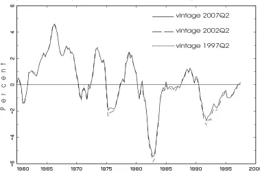
Figure 2 compares one-sided estimates of output gaps over time for three different
vintages. While the dashed line in Figure 1 shows the output gap series estimated from
the latest available vintage of data. Figure 2 traces estimated output gaps obtained
for the time period from 1959Q4 to 1997Q1 from three specific vintages. In contrast to
Figure 1 along a specific line only one unchanged time series for inflation and output
is used in the estimation. The solid line shows output gap estimates using the data
set from 2007Q2, the dashed line from 2002Q2, and the dotted line from 1997Q2. The
data sets differ to the extent to which the data has been revised and in the number
of observations which is higher for younger vintages. The low points of the business
cycle tend to be more pronounced for shorter data sets with less revisions. As we move
to the right and approach the final observation of each data set the estimates diverge
more strongly since data revisions are more pronounced close to the release date of the
data.7
« insert Figure 2 »
Figure 3 presents the inflation forecast which is used together with the forecast for the
output gap in the estimation of the forward-looking Taylor rule. The top panel shows
actual inflation together with the inflation forecast. Forecast errors are presented in
the bottom panel. The RMSE of the inflation forecast is 0.039.
7
« insert Figure 3 »
The next two figures display graphs of the recursive estimates of some of the
hyperpa-rameters of the model and show how the estimated pahyperpa-rameters of the economic model
(12) and (13) change as additional and more accurate data becomes available. Figure
4 contains estimates of the autoregressive coefficients on the output gap φ1 and φ2 and
of the drift of potential outputµy. The dashed lines are bands of 1.96 standard
devia-tions around the point estimates. All parameter estimates are statistically significant
throughout. Both autoregressive parameters are relatively stable over time and are
highly correlated. As shown in the bottom right panel their sum is is roughly constant
and highly significant.
« insert Figure 4 »
Of special interest is the Phillips-curve parameter γ which describes the effect of the output gap on the change in the inflation rate. Figure 5 shows the recursive estimate of
γ together with error bands of 1.96 standard deviations. Except for two short episodes in the 1970s and in the mid-1980s the Phillips-curve coefficient is significantly different
from zero. The size of the effect of the output gap on the change inflation is relatively
low with estimates between 0.02 and 0.03 from the mid 1980s up to the present.
« insert Figure 5 »
Figure 6 displays the recursive one-sided estimates of the coefficients in the Taylor rule.
Often the coefficient on the inflation forecast (upper right panel) is less than one thus
violating the Taylor principle (Taylor (1999)). It sometimes even becomes negative, for
example in the mid-1970s, the mid-1990s and after the bursting of the new economy
bubble in 2001. The coefficient on the output gap (lower left panel) trends upward from
the mid 1980s on but exhibits pronounced cyclical swings. The intercept is extremely
high in the high-inflation era of the 1970s and in the early 1980s.8
« insert Figure 6 »
8
5
Federal Funds Rate forecast uncertainty
5.1
The one-period ahead interest-rate forecast
Forecast uncertainty about the Federal Funds Rate in the next quarter is defined as
Et
(it+1−ˆit+1|t)2|Ωt
. (16)
Definebt= (β0,t βπ,t βz,t ρt)′ and xt = (1 πt+2|t−1 zt+2|t−1 it−1)′, then
ˆit+1|t =Et[it+1|Ωt] =Et
x′t+1bt+1|Ωt
. (17)
Ωt represents the information available to market participants immediately after the
interest rate is set at time t. This information set consists of the estimated reaction function in (3) - (7), of the estimated output gap/inflation model in (12) and (13), and
of the series of current and past interest rates and output gap and inflation forecasts.
Sinceb andx are uncorrelated the one-step ahead forecast for the Federal Funds Rate is
ˆit+1|t=Et
x′t+1|Ωt
Et[bt+1|Ωt] = ˆx′t+1|tbt+1|t. (18)
Note that since xt= (1 πt+2|t−1 zt+2|t−1 it−1)′, the forecast of xt+1 based on Ωt, is
ˆ
xt+1|t = (1 πt+3|t−1 zt+3|t−1 it)′. However the forecast of bt+1 based on Ωt is bt+1|t
asit is part of the information set in periodt.
Combining (16), (17) and (18) leads to
Et
(it+1−ˆit+1|t)2|Ωt
= Et
(x′t+1bt+1−xˆ′t+1|tbt+1|t)2|Ωt
= ˆx′t+1|tPb,t+1|txˆ′t+1|t+b ′
t+1|tPx,t+1|tbt+1|t+σǫ,t2 +1|t. (19)
Pb,t+1|t =Et
(bt+1−bt+1|t)(bt+1−bt+1|t)′
is obtained from the Kalman filter. The first
to possible changes in the Fed’s reaction function.
Px,t+1|t = Et
(xt+1−xt+1|t)(xt+1−xt+1|t)′|Ωt
represents uncertainty about the
fore-cast of the economic variables the interest rate responds to. A detailed derivation of this
expression can be found in Appendix C. The last term in (19) represents uncertainty
caused by the Taylor-rule residual ǫ with σǫ,t2 +1|t being the forecast of the variance of the approximation error using the estimated GARCH coefficients.
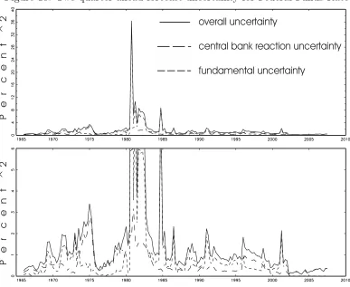
The results for the one-quarter ahead forecast uncertainty in (19) are presented in
Figure 7. The solid line represents aggregate interest rate uncertainty while the other
two lines represent uncertainty about the reaction coefficients in the Taylor rule (long
dashes, first term in (19)) and uncertainty about economic fundamentals in the next
quarter (short dashes, second term in (19)).
« insert Figure 7 »
Figure 7 indicates considerable changes in uncertainty about one-quarter ahead
fore-casts of the Federal Funds Rate. Peaks in forecast uncertainty were in the mid 1970s, in
the early 1980s, in 1984Q4 and in 2002Q2. The lower panel shows a truncated version
of the graph excluding the very high estimated uncertainty in 1980Q3. Even without
looking at the extreme values in the early 1980s, uncertainty about the
one-quarter-ahead Federal Funds Rate was much higher in the 1970s and 1980s than in the 1990s
and 2000s.
The first strong increase in uncertainty in the early 1970s is dominated by rising
un-certainty about the reaction coefficients in the Taylor rule. After a brief decline in the
late 1970s uncertainty about future reaction function coefficients increases once more
after 1977 and remains high up to the early 1980s. The extreme hike in forecast
uncer-tainty in the early 1980s, however, can only partially explained by unceruncer-tainty about
the coefficients in the Fed’s reaction function. Its primary cause is a strong increase
in residual uncertainty, i.e. a massive deterioration of Taylor rule’s ability to track the
actual Federal Funds Rate.9
The same applies to the peak in uncertainty in 1984Q4.
Uncertainty about future economic fundamentals, i.e. output gap and inflation
fore-casts, increases only moderately in the mid-1970s. It remains relatively low throughout
9
the remainder of the sample period. While uncertainty about the Taylor rule
coeffi-cients and uncertainty about future fundamentals are of similar magnitude from the
late 1980s on, the first uncertainty component is quantitatively much more important
in the preceding part of the sample period.
The observed decline in macroeconomic volatility in the U.S. since the mid-1980s has
been attributed to various sources: a decline in the size and frequency of exogenous
shocks, changes in the structure of the U.S. economy, and improvements in monetary
policy, e.g. by enhanced transparency (e.g. Gordon (2005), Stock and Watson (2003)).
The results in this paper shed some light on the relative importance of these
expla-nations by highlighting changes in the predictability of economic fundamentals and
monetary policy in the U.S. Fewer and smaller shocks or a smaller impact of shocks
on the economy due to changes in the economic structure would lead to a smaller
fore-cast uncertainty about future output gaps and inflation. A more systematic and thus
more predictable monetary policy would result in a decline in uncertainty about the
approximation error and uncertainty about the coefficients in the Fed’s policy rule.
Figure 8 graphs one-step-ahead Federal Funds Rate forecasts and forecast errors from
the estimated time-varying Taylor rule. Clearly, forecast errors for the Federal Funds
Rate have been much smaller since 1985 than before (RMSE: post-1985: 0.43, pre-1985:
1.46).
« insert Figure 8 »
Figure 9 shows the time series for uncertainty about fundamentals and uncertainty
about the monetary policy reaction function in greater detail. The top panel displays
the results for uncertainty about future economic fundamentals. Forecast uncertainty
about the output gap and inflation in the late 1980s and in the 1990s is not
consis-tently smaller than before, in particular if compared to the late 1970s and the early
1980s. Uncertainty about fundamentals dropped almost to zero in the mid 1980s but
rose again at the start of the 1990s. Throughout the 1990s it follows a declining trend
interrupted by a brief hike in 1995. In 2001 uncertainty about economic fundamentals
increased again. As far as uncertainty about future output gaps and inflation is
« insert Figure 9 »
The lower panel shows the time series for uncertainty about the coefficients in the
Fed’s reaction function and overall uncertainty about the reaction function. The latter
is defined as the sum of coefficient uncertainty and uncertainty about the approximation
error, i.e. the Taylor rule residual varianceσǫ,t2 . The lower panel uses a scale different from the upper one. For much of the time the two graphs are very close to each other.
The residual variance component becomes important in times when the Taylor rule
does not render a plausible description of monetary policy, particularly in the early
1980s in 1985 and in 2001. The results shown in this panel are consistent with a
quick and persistent decline in uncertainty about the Fed’s reaction function taking
place in the early to mid 1980s. Uncertainty about monetary policy was extremely
low throughout the 1990s and only rose slightly after 2001. The hike in uncertainty
about the Fed’s reaction function in 2001 is due to the high Taylor-rule residual caused
by the Fed drastically lowering the Federal Funds Rate after the bursting of the New
Economy bubble. Overall, the results in Figure 9 show the “good policy” argument
being more important than “good luck”: The predictability of the Fed’s monetary
policy improved strongly and persistently in the mid-1980s while there is no evidence
for such an improvement in forecast uncertainty about economic fundamentals.
5.2
The two-period ahead interest-rate forecast
Uncertainty about the two-quarters ahead forecast of the Federal Funds Rate is
Et
(it+2−ˆit+2|t)2|Ωt
, (20)
where
ˆit+2|t = Et[it+2|Ωt] =Et
x′t+2bt+2|Ωt
(21)
= Et
x′t+2|Ωt
Et
(it+2−ˆit+2|t)2|Ωt
= Et
(x′t+2bt+2−xˆ′t+2|tbt+2|t)2|Ωt
= ˆx′t+2|tPb,t+2|txˆ′t+2|t+b′t+2|tPx,t+2|tb′t+2|t+σǫ,t2 +2|t. (22)
Pb,t+2|t = Et
(bt+2−bt+2|t)(bt+2−bt+2|t)′|Ωt
can be computed as Pb,t+2|t = Pb,t+1|t+
Σw,t+1|t. For the derivation of Px,t+2|t refer to Appendix C.
As expected, the results for (22) shown in Figure 10 demonstrate forecast uncertainty
over two quarters to be generally higher than that over one quarter. The relative
importance of residual uncertainty declines while uncertainty about future economic
fundamentals becomes more important in explaining periods of high forecast
uncer-tainty. Uncertainty about the Taylor rule coefficients is still the main cause for the
increase in overall forecast uncertainty in the mid-1970s and around 1980. For the
longer forecast horizon uncertainty about output gap and inflation forecasts is
quanti-tatively more important than uncertainty about the future policy reaction function for
most of the time after 1980.
« insert Figure 10 »
6
Conclusion
This paper has presented a simple model of monetary policy in the U.S. that separates
the forecast uncertainty about future values of the Federal Funds Rate into uncertainty
about the state of the economy in the future and uncertainty about how the central
bank will react to it.
The results from real-time U.S. data indicate important time variation in the
parame-ters of the policy rule as well as marked changes in the components of Federal Funds
rate forecast uncertainty. In particular, uncertainty about the strength of the Fed’s
future responses to economic fundamentals changed drastically through time and was
most pronounced in mid-1970s and from the late 1970s through the early 1980s. For
a forecast horizon of one quarter, uncertainty about future output gaps and inflation
longer forecast horizon its contribution to forecast uncertainty becomes relatively more
important.
Results focusing on changes in the predictability of future output gaps and inflation
and of the Fed’s monetary policy show uncertainty about monetary policy falling to
unprecedented low levels in the mid 1980s and remaining very low while uncertainty
about economic fundamentals declined only temporarily in the late 1980s. This points
to an important role of increased predictability of monetary policy in the U.S. in
Appendix A: The State-space model for output and
inflation
The observation equation (12) is
Yt =µ+Hx˜t+et, (A1)
with
Yt =
⎡
⎣
∆yt
∆πt
⎤
⎦, µ= ⎡
⎣
µy
0
⎤
⎦, et=
⎡ ⎣ en t 0 ⎤ ⎦ H = ⎡ ⎣
1 −1 0 0 0 0 0 γ 1 δ1 δ2 δ3
⎤
⎦
Eete′t= ΣY =
⎡
⎣
σ2e,n 0
0 0
⎤
⎦,
The transition equation for the state variables can be written as
˜
xt+1 =Fx˜t+ζt+1, (A2)
with
˜
xt =
zt zt−1 νt νt−1 νt−2 νt−3
′
,
ζt =
ezt 0 eνt 0 0 0
′
F = ⎡ ⎢ ⎢ ⎢ ⎢ ⎢ ⎢ ⎢ ⎢ ⎢ ⎢ ⎢ ⎢ ⎣
φ1 φ2 0 0 0 0
1 0 0 0 0 0
0 0 0 0 0 0
0 0 1 0 0 0
0 0 0 1 0 0
0 0 0 0 1 0
⎤ ⎥ ⎥ ⎥ ⎥ ⎥ ⎥ ⎥ ⎥ ⎥ ⎥ ⎥ ⎥ ⎦
Eζtζt′ = Σζ =
⎡ ⎢ ⎢ ⎢ ⎢ ⎢ ⎢ ⎢ ⎢ ⎢ ⎢ ⎢ ⎢ ⎣
σ2e,z 0 0 0 0 0
0 0 0 0 0 0
0 0 σe,ν2 0 0 0
0 0 0 0 0 0
0 0 0 0 0 0
0 0 0 0 0 0
⎤ ⎥ ⎥ ⎥ ⎥ ⎥ ⎥ ⎥ ⎥ ⎥ ⎥ ⎥ ⎥ ⎦ .
The shockseν, en and ez are assumed to be serially and mutually uncorrelated.
Appendix B: The linearized state-space model for the
Taylor rule
After replacing the expectations of the output gap and inflation rate with the
model-generated forecasts the Taylor rule becomes
it=β0,t+βπ,tπt+2|t−1+βz,tzt+2|t−1+f(it−1, βρ,t) +ǫt, (B1)
with
f(it−1, βρ,t) =
1
1 + exp(−βρ,t)
it−1 ≡ρtit−1,
where
βt= (β0,t βπ,t βz,t βρ,t)′.
The Kalman filter is applied to a linearized version of (B1) (see Harvey et al. (1992)):
A linear Taylor approximation to (B1) aroundβρ,t =βρ,t|t−1 results in
it = β0,t+βπ,tπt+2|t−1+βz,tzt+2|t−1+
1
1 + exp(−βρ,t|t−1)
it−1 (B3)
+ exp(−βρ,t|t−1)it−1 (1 + exp(−βρ,t|t−1))2
(βρ,t−βρ,t|t−1) +ǫt.
This can be written as
˜it=β0,t+βπ,tπt+2|t−1 +βz,tzt+2|t−1+ exp(−βρ,t|t−1)it−1
(1 + exp(−βρ,t|t−1))2
βρ,t+ǫt, (B4)
with
˜it=it− it−1
1 + exp(−βρ,t|t−1)
+ exp(−βρ,t|t−1)it−1 (1 + exp(−βρ,t|t−1))2
βρ,t|t−1.
In each iteration of the Kalman filter there is now an additional step to compute ˜i
using the estimate from the previous estimation β˜ρ,t|t−1.
The modifications that result from the assumption of a GARCH process for the error
term are as shown in Kim and Nelson (2006). The error term is included in the
unobserved component. Thus
˜it = 1 π
t+2|t zt+2|t
exp(−βρ,t|t−1)it−1
(1+exp(−βρ,t|t−1))2 1
⎡
⎣
βt ǫt
⎤
⎦ (B5)
= ˜x′tβ˜t, (B6)
˜
βt=Gβ˜t−1+ ˜wt, (B7)
where G = ⎡ ⎢ ⎢ ⎢ ⎢ ⎢ ⎢ ⎢ ⎢ ⎢ ⎣
1 0 0 0 0 0 1 0 0 0 0 0 1 0 0 0 0 0 1 0 0 0 0 0 0
⎤ ⎥ ⎥ ⎥ ⎥ ⎥ ⎥ ⎥ ⎥ ⎥ ⎦ , (B8) ˜
wt =
wt ǫt
, (B9)
and
Ew˜tw˜′t= Σw,t˜ =
⎡
⎣
Σw 0
0 σǫ,t2
⎤
⎦, (B10)
σǫ,t2 = κ0+κ1ǫ2t−1+κ2σ2ǫ,t−2. (B11)
The forecasting equations of the Kalman filter become
˜
βt|t−1 = Gβ˜t−1|t−1, (B12)
Pβ,t˜ |t−1 = GPβ,t˜ −1|t−1G
′ + Σ
˜
w,t. (B13)
After it is observed the estimates are updated as
˜
βt|t = ˜βt|t−1+Pβ,t˜ |t−1x˜t[˜x′tPβ,t˜ |t−1x˜t]−1(˜it−x˜′tβ˜t|t−1), (B14)
Pβ,t˜ |t = Pβ,t˜ |t−1−Pβ,t˜ |t−1x˜t[˜xt′Pβ,t˜ |t−1x˜t]−1x˜′tPβ,t˜ |t−1. (B15)
The covariance matrix of the unobserved statesPβ˜is based onβ˜= (β0,t βπ,t βz,t βρ,t)′.
Appendix C: Uncertainty measures
Uncertainty about economic conditions in the one-period case
Derivation of (19):
Et
(it+1−ˆit+1|t)2|Ωt
= Et
(x′t+1bt+1−xˆ′t+1|tbt+1|t)2|Ωt
= Et
b′t+1xt+1x′t+1bt+1|Ωt
−b′t+1|txˆt+1|txˆ′t+1|tbt+1|t
+σǫ,t2 +1|t (C1)
I use a Taylor-Approximation to write
Eb′t+1xt+1x′t+1bt+1|Ωt
≈ b′t+1|txˆt+1|txˆ′t+1|tbt+1|t (C2)
+ˆx′t+1|tE
(bt+1−bt+1|t)(bt+1−bt+1|t)′|Ωt
ˆ
xt+1|t
+b′t+1|tE
(xt+1−xˆt+1|t)(xt+1−xˆt+1|t)′|Ωt
bt+1|t.
Substituting this expression into (C1) yields (19)
Et
(it+1−ˆit+1|t)2|Ωt
= ˆx′t+1|tEt
(bt+1−bt+1|t)(bt+1−bt+1|t)′|Ωt
ˆ
xt+1|t
+b′t+1|tEt
(xt+1−xˆt+1|t)(xt+1−xˆt+1|t)′|Ωt
bt+1|t
+σǫ,t2 +1|t
= ˆx′t+1|tPb,t+1|txˆ′t+1|t+bt′+1|tPx,t+1|tbt+1|t+σǫ,t2 +1|t, (C3)
with Pb,t+1|t =Et
(bt+1−bt+1|t)(bt+1−bt+1|t)′
and
Px,t+1|t=Et
(xt+1−xt+1|t)(xt+1−xt+1|t)′|Ωt
.
Px,t+1|t = Et
(xt+1−xˆt+1|t)(xt+1−xˆt+1|t)′|Ωt
= ⎡ ⎢ ⎢ ⎢ ⎢ ⎢ ⎢ ⎣
0 0 0 0
0 pπ,π,t+1 pπ,z,t+1 0
0 pπ,z,t+1 pz,z,t+1 0
0 0 0 0
⎤ ⎥ ⎥ ⎥ ⎥ ⎥ ⎥ ⎦ , (C4)
where pπ,π,t+1 =E
(πt+3|t−πt+3|t−1)2|Ωt
, pz,z,t+1 =E
(zt+3|t−zt+3|t−1)2|Ωt
,
and pπ,z,t+1=E
(πt+3|t−πt+3|t−1)(zt+3|t−zt+3|t−1)|Ωt
.
The individual elements can be derived as follows: The inflation forecast the central
bank will react to in the next period is πt+3|t = πt−1 + ∆πt + 3i=1∆πt+i|t while
the forecast of this variable based on information dated t −1 is πt+3|t−1 = πt−1 +
3
i=0∆πt+i|t−1. Hence, using (A1) the forecast error is
πt+3|t−πt+3|t−1 = = (∆πt−∆πt|t−1) + 3
i=1
(∆πt+i|t−∆πt+i|t−1)
= 1′2
(Yt−Yt|t−1) + 3
i=1
(Yt+i|t−Yt+i|t−1)
= 1′2
H(˜xt−x˜t|t−1) +et+
3
i=1
H(˜xt+i|t−x˜t+i|t−1)
(C5)
= 1′2
H(˜xt−x˜t|t−1) +et+H(F +F F +F F F)(˜xt|t−x˜t|t−1)
,
with 12 = (0 1)′.
At the time the policy rate in period t is announced, uncertainty about πt+3|t, the
estimate of inflation the central bank will react to in the next period stems from two
sources: First,(∆πt−∆πt|t−1)is the error made in estimating the change in the inflation
rate from the previous to the current period. Second,3
i=1(∆πt+i|t−∆πt+i|t−1) is the
difference between the changes in inflation from period t+ 1 to t+ 3 as forecast by the central bank at the time it has to set it+1 – and thus formed with knowledge of
Use of the Kalman-filter updating equations results in
πt+3|t−πt+3|t−1 = 1′2
H(˜xt−x˜t|t−1) +et+H(F +F F +F F F)Kt|t−1(H(˜xt−x˜t|t−1)
+et)
= 1′2
H(I+ (F +F F +F F F)Kt|t−1H)(˜xt−x˜t|t−1) (C6)
+(I+H(F +F F +F F F)Kt|t−1)et
,
with Kt|t−1 =Px,t˜ |t−1H′
HP˜x,t|t−1H′+ ΣY
−1
. This can be written as
πt+3|t−πt+3|t−1 = 1′2
D1,x˜(˜xt−x˜t|t−1) +D1,etet
. (C7)
Using this expression the result for pπ,π,t+1 is
pπ,π,t+1 = E
(πt+3|t−πt+3|t−1)2|Ωt
= 1′2
D1,˜xPx,t˜ |t−1D′1,˜x+D1,etΣYD
′
1,et
12. (C8)
zt+3|t is the (1,1) element of x˜t+3|t = F F Fx˜t|t, while zt+3|t−1 is the (1,1) element of
˜
xt+3|t−1 =F F Fx˜t|t−1. Hence,
zt+3|t−zt+3|t−1 = 11′F F F(˜xt|t−x˜t|t−1)
= 1′1F F F Kt|t−1(H(˜xt−x˜t|t−1) +et), (C9)
where the last step makes use of the Kalman filter updating equation for x˜.
Defining
zt+3|t−zt+3|t−1 = 1′1
B1,˜x(˜xt−x˜t|t−1) +B1,etet
, (C10)
pz,z,t+1 = E
(zt+3|t−zt+3|t−1)2|Ωt
= 1′1E
(˜xt+1|t−x˜t+1|t−1)(˜xt+1|t−x˜t+1|t−1)′|Ωt
11
= 1′1
B1,x˜Px,t˜ |t−1B1′,x˜+B1,etΣYB
′
1,et
11, (C11)
with 11 = (1 0 0 0 0 0)′. Uncertainty about the central bank’s forecast for the
output gap is due to the fact that when policy is set next period additional information
in form of observations of πt and yt will be available.
Finally, combining (C7) with (C10) yields
pπ,z,t+1 = E
(πt+3|t−πt+3|t−1)(zt+3|t−zt+3|t−1)|Ωt
= 1′2
D1,x˜Px,t˜ |t−1B1′,x˜+D1,etΣYB
′
1,et
11. (C12)
All these expressions can be evaluated using the parameter estimates from section 3
and the results from the Kalman filter algorithm applied to the model from Appendix
A.
Uncertainty about economic conditions in the two-period case
(22) in the paper is derived analogous to (19). To evaluate (22) the following expression
is required
Px,t+2|t = Et
(xt+2−xˆt+2|t)(xt+2−xˆt+2|t)′|Ωt
= ⎡ ⎢ ⎢ ⎢ ⎢ ⎢ ⎢ ⎣
0 0 0 0
0 pπ,π,t+2 pπ,z,t+2 pπ,i,t+2
0 pπ,z,t+2 pz,z,t+2 pi,z,t+2
0 pπ,i,t+2 pi,z,t+2 pi,i,t+2
where
pπ,π,t+2 = E
(πt+4|t+1−πt+4|t−1)2|Ωt
,
pz,z,t+2 = E
(zt+4|t+1−zt+4|t)2|Ωt
,
pπ,z,t+2 = E
(πt+4|t+1−πt+4|t−1)(zt+4|t+1−zt+4|t)|Ωt
,
pi,i,t+2 = E
(it+1−ˆit+1|t)2|Ωt
,
pπ,i,t+2 = E
(πt+4|t+1−πt+4|t−1)(it+1−ˆit+1|t)|Ωt
,
pi,z,t+2 = E
(it+1−ˆit+1|t)(zt+4|t+1−zt+4|t)|Ωt
.
The inflation forecast the central bank will react to two periods in the future is
πt+4|t+1 =πt−1+ ∆πt+ ∆πt+1+4i=2∆πt+i|t+1,
while πt+4|t−1 =πt−1+ ∆πt|t−1 + ∆πt+1|t−1+4i=2∆πt+i|t−1. Thus,
πt+4|t+1−πt+4|t−1 = (∆πt−∆πt|t−1) + (∆πt+1−∆πt+1|t−1)
+
4
i=2
(∆πt+i|t+1−∆πt+i|t−1)
= 1′2
(Yt−Yt|t−1) + (Yt+1−Yt+1|t−1) + 4
i=2
(Yt+2|t+1−Yt+2|t−1)
= 1′2
H(˜xt−x˜t|t−1) +et+H(˜xt+1−x˜t+1|t−1) +et+1
+
4
i=2
H(˜xt+i|t+1−x˜t+i|t−1)
= 1′2
H(˜xt−x˜t|t−1) +et+H(˜xt+1−x˜t+1|t−1)
+et+1+H(F +F F +F F F)(˜xt+1|t+1−x˜t+1|t−1)
= 1′2
H(˜xt−x˜t|t−1) +et+H(˜xt+1−x˜t+1|t−1) +et+1
+H(F +F F +F F F)(˜xt+1|t+1−x˜t+1|t
+F(˜xt|t−x˜t|t−1))
, (C14)
with12 = (0 1)′ and using the fact that(Yt−Yt|t−1) = H(˜xt−x˜t|t−1) +et Using (12)
πt+4|t+1−πt+4|t−1 = 1′2
H(˜xt−x˜t|t−1) +et+H(F(˜xt−x˜t|t−1) +ζt+1)
+et+1
+H(F +F F +F F F)[Kt+1|t(H(˜xt+1−x˜t+1|t) +et+1)
+F Kt|t−1(H(˜xt−x˜t|t−1) +et))]
πt+4|t+1−πt+4|t−1 = 1′2
H(I+F + (F +F F +F F F)[Kt+1|t(HF(I −Kt|t−1H))
+F Kt|t−1H])(˜xt−x˜t|t−1)
+(I+H(F +F F +F F F)(F Kt|t−1−Kt+1|tHF Kt|t−1))et
+(I+H(F +F F +F F F)Kt+1|t)et+1 (C15)
+H(I+ (F +F F +F F F)Kt+1|tH)ζt+1
.
Define
πt+4|t+1−πt+4|t−1 = 1′2
D2,x˜(˜xt−x˜t|t−1) +D2,etet+D2,et+1et+1 (C16)
+D2,ζζt+1
,
where the respective coefficients are shown in (C15). This leads to
pπ,π,t+2 = E
(πt+4|t+1−πt+4|t−1)2|Ωt
(C17)
= 1′2
D2,˜xPx,t˜ |t−1D′2,˜x+D2,etΣYD
′
2,et +D2,et+1ΣYD ′
2,et+1+D2,ζΣζD ′
2,ζ
12.
zt+4|t+1is the (1,1) element ofx˜t+4|t+1 =F F Fx˜t+1|t+1, whilezt+4|t−1 is the (1,1) element
zt+4|t+1−zt+4|t−1 = 1′1F F F(˜xt+1|t+1−x˜t+1|t−1)
= 1′1F F F(˜xt+1|t+1−x˜t+1|t+ ˜xt+1|t−x˜t+1|t−1)
= 1′1
F F F[Kt+1|tHF(I−Kt|t−1H) +F Kt|t−1H](˜xt−x˜t|t−1)
+F F F[F Kt|t−1−Kt+1|tHF Kt|t−1]et
+F F F Kt+1|tet+1+F F F Kt+1|tHζz+1
. (C18)
Define
zt+4|t+1−zt+4|t−1 = 1′1
B2,x˜(˜xt−x˜t|t−1) +B2,etet+B2,et+1et+1 (C19)
+B2,ζζt+1
,
with the respective coefficients shown in (C18). Hence
pz,z,t+2 = E
(zt+4|t+1−zt+4|t−1)2|Ωt
(C20)
= 1′1E
B2,˜xPx,t˜ |t−1B2′,x˜+B2,etΣYB
′
2,et+B2,et+1ΣYB ′
2,et+1+B2,ζΣζB ′
2,ζ
11.
From (C16) and (C19) it follows that
pπ,z,t+2 = E
(πt+4|t+1−πt+4|t−1)(zt+4|t+1−zt+4|t−1)|Ωt
(C21)
= 1′2
D2,x˜P˜x,t|t−1B2′,x˜+D2,etΣYB
′
2,et+D2,et+1ΣYB ′
2,et+1+D2,ζΣζB ′
2,ζ
11.
Next are the correlations of the forecast errors for the output gap and inflation with
the forecast error for the interest rate. The latter one is
it+1−ˆit+1|t = x′t+1bt+1−xˆ′t+1|tbt+1|t+ǫt+1
= x′t+1(bt+vt+1)−xˆ′t+1|tbt|t+ǫt+1
with vt being the vector of innovations to the Taylor rule coefficients. The first three
elements of v are the first three innovations in wt in (5) with the fourth being the
innovation to ρt.
Since x′t+1 = (1 πt+3|t zt+3|t it) and xˆt′+3|t = (1 πt+3|t−1 zt+3|t−1 it) the above
expression can be expanded to
it+1−ˆit+1|t = (πt+3|t−πt+3|t−1)βπ,t|t+ (zt+3|t−zt+3|t−1)βz,t|t
+(β0,t−β0,t|t) +πt+3|t(βπ,t−βπ,t|t)
+zt+3|t(βz,t−βz,t|t) +it(ρt−ρt|t)
+x′t+1vt+1+ǫt+1. (C23)
The inflation forecast made in period t+ 1 is
πt+3|t = πt−1+ ∆πt+
3
i=1
∆πt+i|t
= πt−1+1′2
4µ+H(I−Kt|t−1H+ (I+F +F F +F F F)Kt|t−1H)
(˜xt−x˜t|t−1) + (I−HKt|t−1+H(I+F +F F +F F F)Kt|t−1)et
+H(I+F +F F +F F F)˜xt|t−1
, (C24)
and (πt+3|t−πt+3|t−1) is shown in (C7).
zt+3|t = 1′1x˜t+3|t
= 1′1F F Fx˜t|t
= 1′1F F F(˜xt|t−1+Kt|t−1(H(˜xt−x˜t|t−1) +et))
= 1′1
F F F Kt|t−1H(˜xt−x˜t|t−1) +F F F Kt|t−1et+F F Fx˜t|t−1
, (C25)
pπ,i,t+2 = E
(πt+4|t+1−πt+4|t−1)(it+1−it+1|t)|Ωt
= 1′2
D2,x˜Px,t˜ |t−1D1′,x˜βπt|t +D2,etΣYD
′
1,etβπt|t
12, (C26)
+1′2
D2,˜xPx,t˜ |t−1B1′,˜xβzt|t +D2,etΣYB
′
1,etβzt|t
11,
and
pi,z,t+2 = E
(zt+4|t+1−zt+4|t−1)(it+1−it+1|t)|Ωt
= 1′1
B2,x˜P˜x,t|t−1D′1,x˜βπt|t +B2,etΣYD
′
1,etβπt|t
12, (C27)
+1′1
B2,x˜Px,t˜ |t−1B1′,x˜βzt|t +B2,etΣYB
′
1,etβzt|t
11.
Finally, pi,i =E
(it+1|t−ˆit+1|t−1)2|Ωt
is known from the one-step-ahead forecast
References
Assenmacher-Wesche, K. "Estimating Central Banks’ Preferences from a Time-varying
Empirical Reaction Function." European Economic Review, 50 (2006),
1951-1974.
Ayuso, J.; A. G. Haldane; and F. Restoy. "Volatility Transmission along the Money
Market Yield Curve." Review of World Economics/ Weltwirtschaftliches Archiv
133 (1997), 56-75.
Boivin, Jean (2006), Has US Monetary Policy Changed? Evidence from Drifting
Coefficients and Real-Time-Data, Journal of Money, Credit, and Banking38(5),
1149-73.
Byrne, Joseph P. and Philip E. Davis (2005), Investment and Uncertainty in the G7,
Review of World Economics/ Weltwirtschaftliches Archiv 141, 1-32.
Caporale, Guglielmo Maria and Andrea Cippolini (2002), The Euro and Monetary
Policy Transparency, Eastern Economic Journal28, 59-70.
Cooley, Thomas and Edward Prescott (1976), Estimation in the Presence of Parameter
Variation, Econometrica 44, 167-84.
Chuderewicz, Russel P. (2002), Using Interest Rate Uncertainty to Predict the
Paper-Bill Spread and Real Output, Journal of Economics and Business 54, 293-312.
Clarida, Richard, Jordi Galí and Mark Gertler (2000), Monetary Policy Rules and
Macroeconomic Stability: Evidence and Some Theory,Quarterly Journal of
Eco-nomics 115, 147-80.
Clark, Peter. K (1989), Trend reversion in real output and unemployment, Journal
of Econometrics 40, 15-32.
Croushore, Dean and Tom Stark (1999), A Real-Time Data Set for Macroeconomists,
Working Paper 99-4, Federal Reserve Bank of Philadelphia.
Croushore, Dean and Tom Stark (2001), A Real-Time Data Set for Macroeconomists,
Croushore, Dean and Tom Stark (2003), A Real-Time Data Set for Macroeconomists:
Does the Data Vintage Matter?, Review of Economics and Statistics 85, 605-17.
European Central Bank (2008), European Central Bank: The First Ten Years,Special
Edition of the Monthly Bulletin, European Central Bank.
Gerberding, Christina, Franz Seitz and Andreas Worms (2005), How the Bundesbank
Really Conducted Monetary Policy, North American Journal of Economics and
Finance 16, 277-92.
Gordon, Robert J. (2005), What caused the decline in U.S. business cycle volatility,
NBER Working Paper 11777.
Hamilton, James. D. (1994), Time Series Analysis, Princeton: Princeton University
Press.
Harvey, A.C., Ruiz, E., and Sentana, E. (1992), "Unobserved Component Time-Series
Models ARCH Disturbances", Journal of Econometrics, 52, 129-157.
Judd, John P. and Glenn D. Rudebusch (1998), Taylor’s Rule and the Fed: 1970-1997.
Federal Reserve Bank of San Francisco Economic Review 1998(3), 3-16.
Kim, Chang-Jin (2006), Time-varying Parameter Models with Endogenous
Regres-sors, Economics Letters 91(1), 21-26.
Kim, Chang-Jin and Charles R. Nelson (1999), State-Space Models with
Regime-Switching - Classical and Gibbs-Sampling Approaches with Applications,
Cam-bridge, MA.: MIT-Press.
Kim, Chang-Jin and Charles R. Nelson (2006), Estimation of a Forward-Looking
Monetary Policy Rule: A Time-Varying Parameter Model using Ex-Post Data,
Journal of Monetary Economics 53, 1949-66.
Kuttner, Kenneth N. (1994), Estimating Potential Output as a Latent Variable,
Jour-nal of Business & Economic Statistics 12(3), 361-368.
Kuzin, Vladimir (2006), The Inflation Aversion of the Bundesbank: A State Space
Approach, Journal of Economic Dynamics and Control 30, 1671-86.
Rate by Mixture Autoregressive Processes, Journal of Financial Econometrics 1,
96-125.
Lansing , Kevin J. (2002), Real-Time Estimation of Trend Output and the Illusion of
Interest Rate Smoothing, Federal Reserve Bank of San Francisco Review, 17-34.
McCulloch, J. Huston (2007), Adaptive Least Squares Estimation of Time-Varying
Taylor Rules, Working Paper, Ohio State University.
Mehra, Yash P. (1999), A Forward-Looking Monetary Policy Reaction Function,
Fed-eral Reserve Bank of Richmond Economic Quarterly 85, 33-53.
Muellbauer, John and Luca Nunziata (2004), Forecasting (and Explaining) US
Busi-ness Cycles, CEPR Discussion Papers 4584.
Nikolsko-Rzhevskyy, Alex (2008), Monetary Policy Evaluation in Real Time:
Forward-Looking Taylor Rules without Forward-Forward-Looking Data, Working Paper, University
of Houston.
Orphanides, Athanasios (2001), Monetary Policy Rules Based on Real-Time Data,
American Economic Review 91, 964-85.
Orphanides, Athanasios (2002), Monetary Policy Rules and the Great Inflation,
Amer-ican Economic Review 92, 115-21.
Orphanides, Athanasios (2003), Monetary Policy Evaluation with Noisy Information,
Journal of Monetary Economics 50, 605-31.
Orphanides, Athanasios and Simon van Norden (2002), The Unreliability of
Output-gap Estimates in Real Time, Review of Economics and Statistics 84, 569-83.
Perez, Stephen J. (2001), Looking Back at Forward-looking Monetary Policy, Journal
of Economics and Business 53, 509-21.
Poole, William (2005), How Predictable is the Fed?, Federal Reserve Bank of St.
Louis Review 87, 659-68.
Reinhart, Vincent R. (2003), Making Monetary Policy in an Uncertain World, in:
Rigobon, Roberto and Brian Sack (2003), Measuring the Reaction of Monetary Policy
to the Stock Market, Quarterly Journal of Economics 118, 639-669.
Stock, James H. and Mark W. Watson (2003), Has the business cycle changed and
why?, in: Gertler, Mark and Kenneth Rogoff (eds.), NBER Macroeconomics
Annual 2002, 17, 159-230.
Sun, Licheng (2005), Regime Shifts in Interest Rate Volatility, Journal of Empirical
Finance 12(3), 418-34.
Taylor, John B. (1993), Discretion versus Policy Rules in Practice,Carnegie-Rochester
Conference Series on Public Policy 39, 195-214.
Taylor, John B. (1999), A Historical Analysis of Monetary Policy Rules, in: Taylor,
John B. (Hrsg.), Monetary Policy Rules, Chicago: The University of Chicago
Press, 319-341.
Tchaidze, Robert R. (2001), Estimating Taylor Rules in a Real Time Setting, Working
Paper, John Hopkins University.
Trecroci, Carmine and Matilde Vassali (2006), Monetary Policy Regime Shifts: New
Evidence from Time-Varying Interest Rate-Rules, Working Paper, University of
Brescia.
Trehan, Bharat and Tao Wu (2004), Time Varying Equilibrium Real Rates and
Mon-etary Policy Analysis, FRBSF Working Paper 2004-10, Federal Reserve Bank of
San Francisco.
Watson, Mark W. (1986), Univariate Detrending Methods with Stochastic Trends,
Figure 1: Output gap estimates from historical and real time data
t
n
e
c
r
e
P
ex-post revised data
real-time data
Figure 2: Output gap estimates from different vintages of real time data
vintage 2007Q2
vintage 2002Q2
vintage 1997Q2
t
n
e
c
r
e
[image:38.612.117.496.428.682.2]Figure 3: Actual inflation and real-time inflation forecasts
ðt ðt|t-2
t
n
e
c
r
e
P
t
n
e
c
r
e
P
Figure 4: Real-time estimates of output-inflation equation coefficients
f2 f1
f +1 f2 m
[image:40.612.124.497.451.703.2]Figure 6: One-sided coefficient estimates
ßß0
ßßz
ßßð
Figure 7: One-quarter ahead forecast uncertainty for Federal Funds Rate
overall uncertainty
central bank reaction uncertainty
fundamental uncertainty
2
^
t
n
e
c
r
e
P
2
^
t
n
e
c
r
e
P
Figure 8: Federal Funds Rate, one-quarter ahead Federal Funds Rate forecasts and
forecast errors
1970 1975 1980 1985 1990 1995 2000 2005
0 4 8 12 16 20
Prozent
1970 1975 1980 1985 1990 1995 2000 2005
−4 −2 0 2 4 6 8
Prozent
FFR
t
FFR
[image:42.612.147.478.446.699.2]Figure 9: Fundamental and monetary policy uncertainty
19650 1970 1975 1980 1985 1990 1995 2000 2005
0.2 0.4 0.6 0.8 1
Prozent
2
uncertainty about future fundamentals
19650 1970 1975 1980 1985 1990 1995 2000 2005
1 2 3
uncertainty about monetary policy
Prozent
2
residual + coefficient uncertainty coefficient uncertainty
Figure 10: Two-quarter ahead forecast uncertainty for Federal Funds Rate
overall uncertainty
central bank reaction uncertainty
fundamental uncertainty
2
^
t
n
e
c
r
e
P
2
^
t
n
e
c
r
e
[image:43.612.118.505.397.714.2]