Munich Personal RePEc Archive
Does the Kyoto Protocol Agreement
matters? An environmental efficiency
analysis
Halkos, George and Tzeremes, Nickolaos
University of Thessaly, Department of Economics
May 2011
Online at
https://mpra.ub.uni-muenchen.de/30652/
Does the Kyoto Protocol Agreement matters?
An environmental efficiency analysis
by
George E. Halkos
*and Nickolaos G. Tzeremes
Department of Economics, University of Thessaly, Korai 43, 38333, Volos, Greece
Abstract
This paper uses both conditional and unconditional Data Envelopment Analysis (DEA) models in order to determine different environmental efficiency levels for a sample of 110 countries in 2007. In order to capture the effect of countries compliance with the Kyoto Protocol Agreement (KPA), we condition the years since a country has signed the agreement until 2007. Particularly, various DEA models have been applied alongside with bootstrap techniques in order to determine the effect of Kyoto protocol agreement on countries’ environmental efficiencies. The study illustrates how the recent developments in efficiency analysis and statistical inference can be applied when evaluating environmental performance issues. The results indicate that the first six years after countries signed the Kyoto protocol agreement have a positive effect on their environmental efficiencies. However after that period it appears that countries avoid complying with the actions imposed by the agreement which in turn has an immediate negative effect on their environmental efficiencies.
Keywords: Environmental efficiency; Kyoto protocol agreement; Conditional full
frontiers; Statistical inference; DEA.
1. Introduction
Input–Output (IO) analysis is a powerful method for analyzing environmental
effects by enabling the calculation of emission multipliers (Östblom, 1998;
Yamakawa and Peters 2009). Other researchers have used environmental computable
general equilibrium (CGE) models in order to analyze environmental effects (Li and
Rose 1995; Ferguson et al. 2005). However, the application of IO analysis to
environmental issues has been applied by several authors (Gale, 1995; Forssell, 1998;
Forssell and Polenske, 1998; Hoekstra and Janssen, 2006. Recently, Washizu and
Nakano (2010) using the Family Income and Expenditure Survey in Japan for 2000,
applied and IO analysis and constructed an eco-efficiency index of consumer
behaviour. In addition Ramon and Cristóbal (2010) developed an environmental IO
linear programming model in order to show how the targets of greenhouse gas (GHG)
emissions set by Kyoto Protocol agreement can be reached.
A special attention has been given to environmental and ecological related
applications of data envelopment analysis (DEA) models in order to find and
investigate efficiency related issues (Halkos and Tzeremes, 2010a). According to
Wier et al. (2005) DEA methodology can be very useful when comparing the
environmental performance of units (in our case countries) by comparing their
eco-efficiency levels (i.e. the lowest possible environmental effect per unit produced).
Many studies have used DEA to assess the environmental performance of a set of
producers by grading their ability to produce the largest equi-proportional increase in
the desirable output and decrease in the undesirable output1 (Zofio and Prieto, 2001).
Färe et al. (1986) were the first to apply classic output oriented DEA analysis
to a set of USA steam electric plants defining radial efficiency measures for
1
equiproportional increases of all outputs (both desirable and undesirable). In addition
they allowed reference technologies to be characterized by strong and weak
disposability of undesirable outputs in order to check for production congestion.
Furthermore, Färe et al. (1989) treated desirable and undesirable production
asymmetrically. They defined efficiency measures that allow desirable and
undesirable outputs to vary by the same proportion but desirable outputs are
proportionally increased while undesirable ones are simultaneously decreased.
Other studies have treated the bad outputs as inputs (Cropper and Oates 1992;
Kopp 1998; Reinhard et al. 1999; Murty and Kumar 2002), while others (Scheel
2001; Seiford and Zhu 2002) have applied a linear monotone decreasing
transformation of the undesirable outputs to be treated as desirable.
In addition to those studies our paper uses conditional full frontiers (Daraio
and Simar, 2005) in order to measure the effect of the Kyoto Protocol Agreement
(KPA)2 for the commitment to CO2 reductions on a sample of 110 countries’
environmental efficiency levels. By applying bootstrap techniques and conditional
measures this paper evaluates countries’ environmental efficiency for 2007. Finally,
additional conditional environmental efficiency indexes are calculated incorporating
the effect of the Kyoto protocol agreement on countries environmental performance in
carbon dioxide emissions.
The structure of the paper is the following. Section 2 presents the data used
while section 3 discusses the proposed methodology. Section 4 comments on the
empirical results derived while the last section concludes the paper.
2
2. Data
Following several studies (Zofio and Prieto 2001; Taskin and Zaim 2000;
Zaim and Taskin 2000; Taskin and Zaim 2001; Zaim 2004; Halkos and Tzeremes
2009; Kumar and Khanna 2009) our paper computes environmental efficiency in CO2
emissions for 110 countries (Appendix-A1). We choose as a desirable output the real
Gross Domestic Product (GDP, expressed in international prices in 2005 US dollar)
and as an undesirable output the CO2 emissions (in millions of tons). The two inputs
considered are aggregate labour input measured by the total employment and total
capital stock3. The two inputs and the desirable output have been obtained from the
Development Data Group, the World Bank (World Bank 2008). The CO2 data have
been obtained from the International Energy Agency-IEA (2010). All the variables
used are for the year 2007.
One of the ways that the bad output can be modelled appeared in the pioneered
work by Färe et al. (1989) by assuming strong (for desirable outputs) and weak (for
undesirable outputs) disposability treated environmental effects as undesirable outputs
in a hyperbolic efficiency measure. Generally the property of weak disposability of
detrimental variables is well known and has been used in several formulations (Färe et
al. 1996, 2004; Chung et al. 1997; Tyteca, 1996, 1997; Zofio and Prieto, 2001; Zhou
et al., 2006, 2007). However, although this approach is widely accepted among the
environmental economists it has faced several criticisms (Hailu and Veeman 2001;
Färe and Grosskopf 2003; Hailu 2003).
3
Another approach for modelling bad output(s) is a linear monotone decreasing
transformation introduced by Seiford and Zhu (2002). Färe and Grosskopf (2004)
commenting on linear monotone decreasing transformation suggested an alternative
approach based on directional output distance function. However, Seiford and Zhu
(2005) replied to the critic made by Färe and Grosskopf (2004) and proved that Färe
and Grosskopf’s proposed model based on directional output distance function is very
similar to the weighted additive model (Ali et al., 1995; Thrall, 1996; Seiford and
Zhu, 1998) where the bad outputs are treated as controllable inputs.
In our DEA setting we treat the bad output (CO2 emissions) as input following
the work by several authors measuring environmental efficiency (Pitman 1981;
Cropper and Oates 1992; Reinhard et al. 2000; Dyckhoff and Allen 2001; Hailu and
Veeman 2001; Korhonen and Luptacik 2004; Tsolas 2005; Weir et al. 2005; Mandal
and Madheswaran 2010). Following those studies we apply a formulation where we
treat undesirable output as input, due to the fact that both traditional inputs and
undesirable output(s) incur costs for countries (Tsolas 2010). According to Mandal
and Madheswaran (2010, p.1110) if the bad outputs are treated as inputs then they
work as a proxy for the use of environment in the form of its assimilative capacity.
Moreover, by applying the methodology introduced by Daraio and Simar
(2005) we conditioned in a second stage the effect of countries commitment to Kyoto
protocol agreement on their environmental efficiencies (for the year 2007). As such
an external variable has been used based on the time distance of the year in which the
country has signed the agreement and the year the environmental efficiency was
computed (i.e. 2007). Under the protocol agreement both developed and developing
pursuing emissions cuts in a wide range of economic sectors. As such by conditioning
the years from the time which the countries have agreed with the actions imposed by
the KPA we will be able to capture that effect on their estimated environmental
efficiencies calculated in the latter period (in our case for 2007). The information
regarding the year in which each country has signed the agreement has been obtained
from the United Nations Framework Convention on Climate Change (2006).
3. Methodology
3.1 Efficiency measurement
Trying to measure countries environmental efficiency in a context described
by Shephard (1970) we define a set of x∈R+p inputs which are used to produce
q
R
y∈ + outputs. Then the feasible combinations of
( )
x,y can be defined as:( )
⎭ ⎬ ⎫ ⎩
⎨
⎧ ∈
=
Ψ +
+ x can produce y
R y
x, p q (1)
In an input oriented case in Farrell’s (1957) context countries’ environmental
efficiency operating at level (x, y) can then be defined as:
( )
x,y =inf{
θ(
θx,y)
∈Ψ}
θ (2)
where an inefficient country working at a level (x, y) in order to increase its efficiency
needs to reduce proportionally its inputs by θ
( )
x,y ≤1. In addition when the countriesare in the efficient frontier then θ
( )
x,y =1.Following Charnes et al. (1978) we assume free disposability and convexity of
the production setΨ. Furthermore, when evaluating the performance of the countries
in terms of their environmental efficiency levels, input orientation of DEA models
have been applied due to the fact that input quantities appear to be the primary
decision variables and therefore the decision makers have most control over the
2011). Following the notation by Daraio and Simar (2007) given a list of p inputs and
q outputs, any productive country can be defined by means of a set of points, Ψ, which forms the production set. Therefore, efficiency measurement of a given country
) ,
(x y relative to the boundary of the convex hull of X =
{
(
Xi,Yi)
,i=1...n}
can becalculated as:
( )
(
)
⎪ ⎪ ⎭ ⎪⎪ ⎬ ⎫ ⎪ ⎪ ⎩ ⎪⎪ ⎨ ⎧ = ≥ = ≥ ≤ ℜ ∈ = Ψ∑
∑
∑
= = = + + ∧ n i i i n i n n i i i i i q p DEA n i t s for X x Y y y x 1 1 1 1 ,..., 1 , 0 ; 1 . . ,..., , ; , γ γ γ γ γ γ (3)The DEA
∧
Ψ in (3) allows for variables returns to scale (VRS) and has been introduced
by Banker et al. (1984). According to Charnes et al. (1978) constant returns to scale
(CRS) is applied when the equality constrained
∑
= = n i i 1 1
γ in (3) is omitted.
For a country operating at a level (x0, y0) the estimation of the input oriented
DEA model is obtained by solving the linear program illustrated below as (4)-(5):
(
)
(
)
⎭ ⎬ ⎫ ⎩ ⎨⎧ ∈Ψ
= ∧
∧
DEA DEA x0,y0 inf θ θx0,y0
θ (4)
(
)
⎪ ⎪ ⎭ ⎪⎪ ⎬ ⎫ ⎪ ⎪ ⎩ ⎪⎪ ⎨ ⎧ = ≥ = ≥ ≥ ≤ =∑
∑
∑
= = = ∧ n i i i n i i i n i i i DEA n i X x Y y y x 1 1 0 1 0 0 0 ,..., 1 ; 0 ; 1 ; 0 ; ; min , γ γ θ γ θ γ θθ (5).
3.2 Efficiency bias correction and confidence intervals construction
According to Simar and Wilson (1998, 2000) DEA efficiency scores are
biased by construction and therefore bootstrap techniques must be applied in order to
eliminate the bias created. They introduced an approach based on bootstrap
indicators (Appendix-A2). The bootstrap bias estimate for the original DEA estimator
) , (x y
DEA ∧
θ can be calculated as:
∑
= ∧ ∧ − ∧ ∧ − = ⎟ ⎠ ⎞ ⎜ ⎝ ⎛ B b DEA b DEA DEAB x y B x y x y
BIAS 1 , * 1 ) , ( ) , ( ) ,
( θ θ
θ
(6).
Furthermore, *DEA,b(x,y) ∧
θ are the bootstrap values and B is the number of
bootstrap replications. Then a biased corrected estimator of θ(x,y) can be calculated
as:
∑
= ∧ − ∧ ∧ ∧ ∧ ∧ ∧ − = ⎟ ⎠ ⎞ ⎜ ⎝ ⎛ − = B b b DEA DEA DEA B DEADEA x y x y BIAS x y x y B x y
1 , * 1 ) , ( ) , ( 2 ) , ( ) , ( ) ,
( θ θ θ θ
θ
(7).
However, according to Simar and Wilson (2008) this bias correction can
create an additional noise and the sample variance of the bootstrap values
) , ( , * y x b DEA ∧
θ has to be calculated. The calculation of the variance of the bootstrap
values is illustrated below:
∑
∑
= = ∧ − ∧ − ∧ ⎥ ⎦ ⎤ ⎢ ⎣ ⎡ − = B b B b b DEA bDEA x y B x y
B 1 2 1 , * 1 , * 1 2 ) , ( ) , ( θ θ σ (8).
Additionally we need to avoid the bias correction illustrated in (7) unless:
3 1 )) , ( ( > ∧ ∧ ∧ σ
θ x y
BIASB DEA
(9).
By expressing the input oriented efficiency in terms of the Shephard’s (1970) input
distance function as ( , ) 1
( , ) DEA DEA x y x y δ θ ∧ ∧
≡ we can construct 95-percent confidence
intervals forδDEA( , )x y
∧
as: δDEA( , )x y α1 a/ 2,δDEA( , )x y αa/ 2
∧ ∧ ∧ ∧
−
⎡ − − ⎤
⎢ ⎥
⎣ ⎦ (10).
In order to choose between the adoption of the results obtained by the CCR
(Charnes et al. 1978) and BCC (Banker et al. 1984) models in terms of the
consistency of our results obtained we adopt the method introduced by Simar and
Wilson (2002). Therefore, we compute the DEA efficiency scores under the CRS and
VRS assumption and by using the bootstrap algorithm described previously we test
for the CRS results against the VRS results obtained such as:
VRS is H against CRS is
Ho :Ψϑ 1:Ψϑ (11)
The test statistic is given by the following equation as:
( )
(
)
(
)
∑
= ∧ ∧ = n i i i i i n Y X n vrs Y X n crs n X T1 , ,
, , 1 θ θ (12)
Then the p-value of the null hypotheses can be approximated by the proportion of
bootstrap samples as:
∑
(
)
= ≤ = − B b obs b B T T I value p 1 *, (13)
where B is 2000 bootstrap replications, I is the indicator function and T*,bare the
bootstrap samples and original observed values are denoted by Tobs.
3.4 Testing the effect of external ‘environmental’ variables on the efficiency scores
In order to analyse the effect the years passed since a country has signed and
adopted the Kyoto protocol agreement (z) on the efficiency scores obtained we follow
the probabilistic approach developed by Daraio and Simar (2005). They suggest that
the joint distribution of (X, Y) conditional on the environmental factor Z=z defines
the production process if Z=z. The efficiency measure can then be defined as:
(
)
{
, 0}
inf ) ,
(x yz = θ FX θxy z >
θ (14)
as follows:
(
)
(
) (
(
)
)
(
y y) (
K(
z z)
h)
I h z z K y y x x I z y x F i n i i n
i i i i
n Z Y X / / , , 1 1 , , − ≥ − ≥ ≤ =
∑
∑
= = ∧ (15)where K(.) is the Epanechnikov kernel4 and h is the bandwidth of appropriate size.
Following, Bădin et al. (2010) we use a fully automatic data-driven approach for
bandwidth selection based on the work of Hall et al. (2004) and Li and Racine (2004;
2007) least-squares cross-validation criterion (LSCV) which leads to bandwidths of
optimal size for the relevant components of Z. This method is based on the principle
of selecting a bandwidth that minimizes the integrated squared error of the resulting
estimate5. Li and Racine (2007) suggest that we have also to correct the resulting h
by an appropriate scaling factor, which is (4 )(4 )
q q r r n
−
+ + +
where qis the dimension of Y
and ris the dimension ofZ6. Therefore, we can obtain a conditional DEA efficiency
measurement defined as:
(
)
(
)
⎭ ⎬ ⎫ ⎩ ⎨ ⎧ > = ∧ ∧ 0 , inf,yz F , , xy z
x XYZn
DEA θ θ
θ (16).
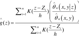
Then in order to establish the influence of an environmental variable on the
efficiency scores obtained a scatter of the ratios
(
)
( )
x y z y x n n , , ∧ ∧ θ θagainst Z (the years since
the Kyoto agreement has been signed by a country) and its smoothed non parametric
regression lines it would help us to analyse the effect of Z on the environmental
efficiency scores obtained. For this purpose we use the nonparametric regression
estimator introduced by Nadaraya (1965) and Watson (1964) as:
4
Other kernels from the family of continuous kernels with compact support can also be used.
5
See Bădin et al. (2010) for a Matlab routine that computes the bandwidth based on the LSCV criterion.
6
(
)
( )
1
1
,
( )
, ( )
( )
n
n i
i
n
n i
i
x y z
z Z
K
h x y
g z
z Z
K h
θ θ ∧
∧ =
∧
=
⎛ ⎞
− ⎜ ⎟
⎜ ⎟
⎜ ⎟
⎝ ⎠
= −
∑
∑
(17).If this regression is increasing it indicates that Z is unfavourable to the
countries’ environmental efficiency whereas if it is decreasing then it is favourable.
When Z is unfavourable then the environmental factor acts like an extra undesired
output to be produced demanding the use of more inputs in the production activity. In
the opposite case the environmental factor plays a role of a substitutive input in the
production process giving the opportunity to save inputs in the activity of production.
4. Empirical Results
Following the methodology proposed by Simar and Wilson (2002) our paper
tests the model for the existence of constant or variable returns to scale (analysed
previously in equations 11-13). In our application we have three input factors and one
outputs and we obtained for this test a p-value of 0.6 > 0.05 (with B=2000) hence, we
cannot reject the null hypothesis of CRS. Therefore, the results adopted in our study
[image:12.595.93.262.73.151.2]are based on the CCR model assuming constant returns to scale7.
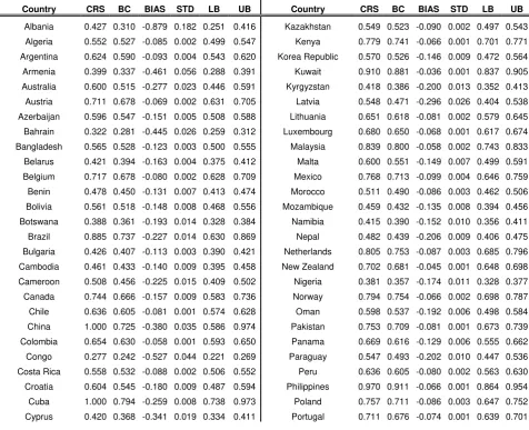
Table 1 provides the results of CRS analysis adopting the correction for bias
using the methodology proposed by Simar and Wilson (1998, 2000). For the sample
of 110 countries under the CRS assumption only four countries appear to be
environmentally efficient (efficiency score = 1). These are China, Cuba, the UK and
the USA. The last ten performers are reported to be Botswana, Zambia, Nigeria,
Estonia, Bahrain, Senegal, Dominican Republic, Honduras, Congo and Togo.
realise that the environmental efficiency scores are in many cases considerably lower
(looking at the descriptive statistics). For instance in the case of the USA the biased
corrected (BC) environmental efficiency score is 0.728 with lower bound (LB) of
0.584 and upper bound (UB) of 0.97 in a confidence interval of 95%. Almost identical
results are reported in the case of China where the biased corrected (BC)
environmental efficiency score is 0.724 with a lower bound (LB) of 0.585 and an
upper bound (UB) of 0.974 in a confidence interval of 95%. Daraio and Simar (2007)
suggest that when the bias (BIAS) is larger than the standard deviation (STD) then the
bias corrected environmental efficiencies (BC) must be preferred compared to the
[image:13.595.59.536.385.772.2]original estimates.
Table 1: Environmental efficiency scores, biased corrected efficiency scores and lower and upper bounds for 95% confidence intervals
Country CRS BC BIAS STD LB UB Country CRS BC BIAS STD LB UB
Albania 0.427 0.310 -0.879 0.182 0.251 0.416 Kazakhstan 0.549 0.523 -0.090 0.002 0.497 0.543
Algeria 0.552 0.527 -0.085 0.002 0.499 0.547 Kenya 0.779 0.741 -0.066 0.001 0.701 0.771
Argentina 0.624 0.590 -0.093 0.004 0.543 0.620 Korea Republic 0.570 0.526 -0.146 0.009 0.472 0.564
Armenia 0.399 0.337 -0.461 0.056 0.288 0.391 Kuwait 0.910 0.881 -0.036 0.001 0.837 0.905
Australia 0.600 0.515 -0.277 0.023 0.446 0.591 Kyrgyzstan 0.418 0.386 -0.200 0.013 0.352 0.413
Austria 0.711 0.678 -0.069 0.002 0.631 0.705 Latvia 0.548 0.471 -0.296 0.026 0.404 0.538
Azerbaijan 0.596 0.547 -0.151 0.005 0.508 0.588 Lithuania 0.651 0.618 -0.081 0.002 0.579 0.645
Bahrain 0.322 0.281 -0.445 0.026 0.259 0.312 Luxembourg 0.680 0.650 -0.068 0.001 0.617 0.674
Bangladesh 0.565 0.528 -0.123 0.003 0.500 0.555 Malaysia 0.839 0.800 -0.058 0.002 0.743 0.833
Belarus 0.421 0.394 -0.163 0.004 0.375 0.412 Malta 0.600 0.551 -0.149 0.007 0.499 0.591
Belgium 0.717 0.678 -0.080 0.002 0.628 0.709 Mexico 0.768 0.713 -0.099 0.004 0.646 0.759
Benin 0.478 0.450 -0.131 0.007 0.413 0.474 Morocco 0.511 0.490 -0.086 0.003 0.462 0.506
Bolivia 0.561 0.518 -0.148 0.008 0.468 0.556 Mozambique 0.459 0.432 -0.135 0.008 0.394 0.456
Botswana 0.388 0.361 -0.193 0.014 0.328 0.384 Namibia 0.415 0.390 -0.152 0.010 0.356 0.411
Brazil 0.885 0.737 -0.227 0.014 0.630 0.869 Nepal 0.482 0.439 -0.206 0.009 0.406 0.475
Bulgaria 0.426 0.407 -0.113 0.003 0.390 0.421 Netherlands 0.805 0.753 -0.087 0.003 0.685 0.796
Cambodia 0.461 0.433 -0.140 0.009 0.395 0.458 New Zealand 0.702 0.681 -0.045 0.001 0.648 0.698
Cameroon 0.508 0.456 -0.225 0.015 0.409 0.502 Nigeria 0.381 0.357 -0.174 0.011 0.328 0.377
Canada 0.744 0.666 -0.157 0.009 0.583 0.736 Norway 0.794 0.754 -0.066 0.002 0.698 0.787
Chile 0.636 0.605 -0.081 0.001 0.574 0.628 Oman 0.598 0.537 -0.192 0.006 0.498 0.584
China 1.000 0.725 -0.380 0.035 0.586 0.974 Pakistan 0.753 0.709 -0.081 0.001 0.673 0.739
Colombia 0.654 0.630 -0.058 0.001 0.593 0.650 Panama 0.669 0.616 -0.129 0.006 0.555 0.662
Congo 0.277 0.242 -0.527 0.044 0.221 0.269 Paraguay 0.547 0.493 -0.202 0.010 0.447 0.536
Costa Rica 0.558 0.532 -0.088 0.002 0.506 0.552 Peru 0.636 0.605 -0.080 0.002 0.563 0.630
Croatia 0.604 0.545 -0.180 0.009 0.487 0.594 Philippines 0.970 0.911 -0.066 0.001 0.864 0.954
Cuba 1.000 0.794 -0.259 0.008 0.738 0.973 Poland 0.757 0.711 -0.086 0.003 0.647 0.752
Czech Republic 0.646 0.615 -0.077 0.001 0.581 0.638 Qatar 0.524 0.419 -0.479 0.050 0.356 0.510
Denmark 0.755 0.723 -0.058 0.001 0.677 0.749 Romania 0.464 0.442 -0.107 0.004 0.415 0.459
Dominican Republic 0.313 0.250 -0.797 0.268 0.203 0.308 Russian Federation 0.763 0.689 -0.141 0.008 0.608 0.754
Ecuador 0.529 0.493 -0.139 0.004 0.464 0.520 Saudi Arabia 0.906 0.854 -0.067 0.001 0.794 0.893
Egypt 0.840 0.808 -0.048 0.001 0.767 0.833 Senegal 0.315 0.285 -0.332 0.029 0.257 0.310
El Salvador 0.673 0.600 -0.180 0.007 0.544 0.662 Singapore 0.559 0.539 -0.066 0.002 0.510 0.555
Eritrea 0.892 0.791 -0.143 0.006 0.697 0.878 Slovak Republic 0.596 0.577 -0.055 0.001 0.551 0.592
Estonia 0.353 0.308 -0.408 0.024 0.282 0.341 Slovenia 0.464 0.432 -0.158 0.005 0.406 0.456
Ethiopia 0.481 0.429 -0.248 0.013 0.391 0.475 South Africa 0.708 0.676 -0.067 0.002 0.630 0.704
Finland 0.785 0.757 -0.048 0.001 0.711 0.781 Spain 0.571 0.509 -0.213 0.016 0.448 0.565
France 0.770 0.660 -0.216 0.015 0.564 0.758 Sri Lanka 0.464 0.422 -0.212 0.007 0.392 0.451
Georgia 0.618 0.564 -0.156 0.004 0.523 0.605 Sudan 0.888 0.860 -0.037 0.000 0.822 0.882
Germany 0.877 0.742 -0.207 0.015 0.620 0.863 Sweden 0.827 0.782 -0.069 0.002 0.727 0.818
Ghana 0.414 0.382 -0.203 0.009 0.352 0.408 Switzerland 0.748 0.710 -0.072 0.002 0.658 0.741
Greece 0.823 0.780 -0.067 0.001 0.731 0.812 Syrian Arab Republic 0.551 0.503 -0.175 0.004 0.471 0.537
Guatemala 0.613 0.548 -0.193 0.007 0.504 0.603 Thailand 0.593 0.567 -0.078 0.002 0.532 0.589
Haiti 0.752 0.711 -0.076 0.003 0.651 0.747 Togo 0.081 0.059 -4.595 5.118 0.048 0.079
Honduras 0.305 0.271 -0.411 0.030 0.248 0.297 Trinidad and Tobago 0.742 0.668 -0.149 0.007 0.596 0.734
Hungary 0.756 0.723 -0.060 0.001 0.688 0.747 Tunisia 0.522 0.490 -0.128 0.004 0.458 0.517
Iceland 0.493 0.457 -0.162 0.006 0.425 0.486 Ukraine 0.587 0.566 -0.062 0.002 0.535 0.583
India 0.487 0.433 -0.258 0.022 0.381 0.480 United Arab Emirates 0.889 0.851 -0.050 0.001 0.802 0.881
Indonesia 0.605 0.560 -0.134 0.008 0.504 0.599 United Kingdom 1.000 0.877 -0.140 0.007 0.751 0.983
Ireland 0.772 0.743 -0.051 0.001 0.697 0.768 USA 1.000 0.728 -0.373 0.035 0.585 0.970
Israel 0.859 0.825 -0.048 0.001 0.782 0.851 Uruguay 0.838 0.797 -0.061 0.001 0.753 0.830
Italy 0.797 0.705 -0.165 0.010 0.611 0.787 Uzbekistan 0.657 0.626 -0.076 0.001 0.594 0.650
Jamaica 0.588 0.514 -0.245 0.020 0.444 0.580 Venezuela 0.840 0.799 -0.061 0.002 0.740 0.835
Japan 0.737 0.597 -0.317 0.031 0.493 0.723 Yemen 0.541 0.466 -0.296 0.015 0.424 0.528
Jordan 0.518 0.482 -0.144 0.006 0.445 0.512 Zambia 0.385 0.354 -0.232 0.017 0.320 0.381
Descriptive Statistics
CRS BC BIAS STD LB UB
Mean 0.628 0.575 -0.209 0.059 0.527 0.620
Std 0.184 0.169 0.445 0.488 0.159 0.181
Min 0.081 0.059 -4.595 0.000 0.048 0.079
Max 1.000 0.911 -0.036 5.118 0.864 0.983
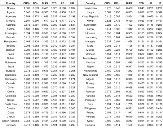
In addition to table 1, table 2 provides the analytical results of countries’
environmental efficiency taking into consideration the number of years since a
country has signed the KPA. Again we test our model for the existence of constant or
variable returns to scale (equations 11-13). The p-value of the test is 0.77 > 0.05 (with
B=2000); hence again we cannot reject the null hypothesis of CRS and the results
obtained from the CCR model have been adopted. The conditional environmental
Following the methodology presented previously the results indicate that the
environmental efficient countries under the effect of the KPA (CRS|z) are Albania,
China, El Salvador, Panama and the USA. The last ten performers are reported to be
Morocco, Poland, Norway, Romania, Slovak Republic, Austria, Korea Republic,
India, Dominican Republic and Togo.
However as previously stated the biased corrected results need to be adopted
since the bias is larger than the standard deviation (Daraio and Simar 2007). Again
great differences are been reported on the conditional environmental efficiencies of
the countries under evaluation (looking at the standard deviations of the conditional
environmental efficiency scores). For instance in the case of the USA the biased
corrected conditional environmental efficiency score (BC|z) is 0.60 with lower bound
of 0.52 and upper bound of 0.91 in a confidence interval of 95%. Therefore, taking
into consideration the biased corrected conditional environmental efficiency scores
the highest ten performers are reported to be Albania, Panama, El Salvador,
Uzbekistan, Pakistan, the USA, China, Egypt, Trinidad and Tobago and Jamaica.
Whereas the ten countries with the lowest biased corrected conditional environmental
efficiency scores are reported to be Romania, Canada, Morocco, Austria, Japan,
Slovak Republic, Korea Republic, India, Dominican Republic and Togo.
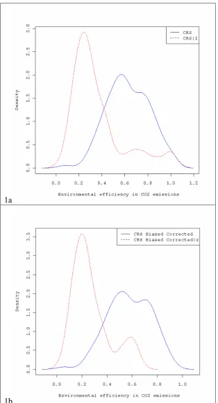
Figure 1 presents the density estimates using the “normal reference
rule-of-thumb” approach for bandwidth selection (Silverman, 1986) and a second order
Gaussian kernel. Subfigure 1a, indicates the differences between the environmental
efficiency scores and the conditional environmental efficiency scores. It appears that
the original estimates under the CRS assumption (solid line) are platykurtic compared
to the original CRS conditional estimates (dotted line) which appear to be leptokurtic.
move away from the mean. Furthermore, the pickedness of the distribution suggests a
clustering around the mean with rapid fall around it. In addition subfigure 1b indicates
high differences between the densities of the biased corrected environmental
efficiency scores (solid line) and the biased corrected conditional efficiency scores
(dotted line). As can be realised the conditional estimates (original and biased
corrected) are reported to be lower compared to the unconditioned environmental
efficiency estimates (original and biased corrected). This in turn indicates that when
we account for the effect of the KPA countries’ environmental efficiency scores tend
[image:16.595.34.561.355.769.2]to decrease rather than to increase.
Table 2: Conditional environmental efficiency scores biased corrected efficiency scores and lower and upper bounds for 95% confidence intervals.
Country CRS|z BC|z BIAS STD LB UB Country CRS|z BC|z BIAS STD LB UB
Albania 1.000 0.673 -0.485 0.025 0.580 0.897 Kazakhstan 0.277 0.247 -0.430 0.045 0.221 0.270
Algeria 0.647 0.524 -0.365 0.031 0.438 0.618 Kenya 0.382 0.290 -0.833 0.080 0.253 0.349
Argentina 0.209 0.172 -1.026 0.227 0.146 0.199 Korea Republic 0.116 0.087 -2.854 1.329 0.075 0.110
Armenia 0.301 0.200 -1.677 0.213 0.177 0.270 Kuwait 0.528 0.432 -0.420 0.023 0.381 0.491
Australia 0.573 0.391 -0.812 0.099 0.328 0.537 Kyrgyzstan 0.223 0.170 -1.403 0.280 0.146 0.210
Austria 0.131 0.106 -1.761 0.618 0.091 0.124 Latvia 0.441 0.302 -1.042 0.104 0.262 0.394
Azerbaijan 0.394 0.328 -0.510 0.045 0.286 0.375 Lithuania 0.353 0.264 -0.955 0.105 0.230 0.324
Bahrain 0.412 0.337 -0.539 0.057 0.289 0.394 Luxembourg 0.323 0.264 -0.689 0.051 0.236 0.298
Bangladesh 0.169 0.138 -1.305 0.216 0.122 0.159 Malaysia 0.237 0.191 -1.026 0.154 0.165 0.221
Belarus 0.298 0.262 -0.450 0.040 0.236 0.287 Malta 0.288 0.214 -1.196 0.158 0.187 0.266
Belgium 0.200 0.173 -0.798 0.189 0.148 0.194 Mexico 0.293 0.238 -0.799 0.237 0.192 0.286
Benin 0.220 0.175 -1.191 0.275 0.147 0.209 Morocco 0.151 0.111 -2.382 0.687 0.095 0.139
Bolivia 0.704 0.497 -0.590 0.060 0.416 0.663 Mozambique 0.409 0.319 -0.686 0.097 0.270 0.394
Botswana 0.244 0.185 -1.316 0.196 0.160 0.222 Namibia 0.254 0.201 -1.040 0.223 0.169 0.245
Brazil 0.280 0.195 -1.573 0.336 0.165 0.261 Nepal 0.432 0.316 -0.847 0.068 0.277 0.392
Bulgaria 0.273 0.234 -0.616 0.054 0.211 0.261 Netherlands 0.160 0.133 -1.243 0.447 0.113 0.155
Cambodia 0.243 0.190 -1.153 0.232 0.161 0.232 New Zealand 0.196 0.162 -1.068 0.145 0.144 0.183
Cameroon 0.288 0.229 -0.891 0.125 0.197 0.271 Nigeria 0.264 0.212 -0.913 0.204 0.178 0.254
Canada 0.153 0.112 -2.388 0.757 0.096 0.143 Norway 0.147 0.119 -1.569 0.475 0.102 0.138
Chile 0.228 0.202 -0.562 0.070 0.181 0.221 Oman 0.363 0.310 -0.468 0.048 0.271 0.350
China 1.000 0.605 -0.652 0.040 0.527 0.894 Pakistan 0.776 0.608 -0.357 0.022 0.512 0.723
Colombia 0.240 0.208 -0.644 0.084 0.183 0.230 Panama 1.000 0.644 -0.552 0.022 0.588 0.909
Congo 0.278 0.207 -1.240 0.143 0.181 0.253 Paraguay 0.675 0.466 -0.662 0.056 0.399 0.633
Costa Rica 0.291 0.229 -0.920 0.107 0.201 0.268 Peru 0.194 0.144 -1.765 0.372 0.125 0.178
Croatia 0.335 0.232 -1.323 0.177 0.202 0.300 Philippines 0.445 0.380 -0.381 0.027 0.335 0.424
Cuba 0.274 0.226 -0.775 0.111 0.196 0.262 Poland 0.151 0.117 -1.947 0.614 0.100 0.141
Dominican Republic 0.090 0.056 -6.652 5.206 0.048 0.083 Russian Federation 0.226 0.177 -1.231 0.458 0.143 0.219
Ecuador 0.356 0.306 -0.462 0.041 0.270 0.342 Saudi Arabia 0.329 0.284 -0.481 0.071 0.243 0.319
Egypt 0.758 0.591 -0.374 0.020 0.507 0.703 Senegal 0.216 0.167 -1.381 0.216 0.145 0.199
El Salvador 1.000 0.621 -0.610 0.030 0.556 0.894 Singapore 0.665 0.526 -0.397 0.030 0.441 0.619
Eritrea 0.539 0.403 -0.623 0.058 0.344 0.505 Slovak Republic 0.131 0.100 -2.318 0.590 0.087 0.118
Estonia 0.265 0.221 -0.765 0.117 0.192 0.255 Slovenia 0.281 0.246 -0.500 0.056 0.219 0.272
Ethiopia 0.370 0.295 -0.683 0.069 0.256 0.345 South Africa 0.441 0.364 -0.480 0.050 0.309 0.416
Finland 0.443 0.369 -0.449 0.042 0.317 0.423 Spain 0.185 0.140 -1.721 0.697 0.116 0.177
France 0.161 0.117 -2.340 0.913 0.098 0.150 Sri Lanka 0.277 0.238 -0.584 0.078 0.209 0.269
Georgia 0.738 0.541 -0.494 0.028 0.470 0.669 Sudan 0.231 0.178 -1.272 0.191 0.156 0.212
Germany 0.184 0.132 -2.160 0.918 0.110 0.176 Sweden 0.191 0.166 -0.809 0.172 0.144 0.185
Ghana 0.313 0.231 -1.140 0.167 0.199 0.291 Switzerland 0.229 0.197 -0.693 0.143 0.169 0.221
Greece 0.175 0.151 -0.925 0.188 0.132 0.169 Syrian Arab Republic 0.449 0.375 -0.437 0.036 0.328 0.429
Guatemala 0.457 0.365 -0.555 0.051 0.314 0.430 Thailand 0.298 0.259 -0.497 0.072 0.224 0.289
Haiti 0.633 0.510 -0.382 0.038 0.423 0.614 Togo 0.040 0.024 -16.310 25.072 0.021 0.036
Honduras 0.327 0.256 -0.846 0.091 0.222 0.305 Trinidad and Tobago 0.878 0.586 -0.567 0.047 0.498 0.835
Hungary 0.160 0.132 -1.317 0.245 0.116 0.150 Tunisia 0.280 0.234 -0.700 0.076 0.208 0.267
Iceland 0.268 0.196 -1.377 0.155 0.172 0.240 Ukraine 0.406 0.348 -0.413 0.037 0.302 0.391
India 0.102 0.072 -4.162 1.932 0.062 0.095 United Arab Emirates 0.311 0.272 -0.454 0.048 0.240 0.299
Indonesia 0.219 0.173 -1.212 0.309 0.145 0.207 United Kingdom 0.209 0.160 -1.456 0.568 0.131 0.202
Ireland 0.430 0.359 -0.459 0.045 0.308 0.409 USA 1.000 0.607 -0.648 0.042 0.526 0.916
Israel 0.218 0.188 -0.725 0.079 0.169 0.208 Uruguay 0.408 0.287 -1.038 0.094 0.251 0.363
Italy 0.166 0.126 -1.924 0.835 0.104 0.159 Uzbekistan 0.902 0.618 -0.509 0.028 0.544 0.823
Jamaica 0.846 0.571 -0.569 0.029 0.512 0.760 Venezuela 0.278 0.232 -0.718 0.108 0.199 0.265
Japan 0.156 0.105 -3.065 1.464 0.089 0.146 Yemen 0.322 0.265 -0.676 0.089 0.228 0.308
Jordan 0.347 0.250 -1.110 0.139 0.217 0.321 Zambia 0.400 0.300 -0.837 0.093 0.257 0.366
Descriptive Statistics
CRS BC BIAS STD LB UB
Mean 0.360 0.273 -1.207 0.498 0.236 0.336
Std 0.229 0.153 1.690 2.432 0.133 0.208
Min 0.040 0.024 -16.310 0.020 0.021 0.036
Figure 1: Kernel density functions of countries’ environmental efficiencies derived from unconditional and conditional CRS and biased corrected CRS DEA models using Gaussian Kernel and the appropriate bandwidth
1a
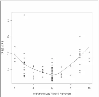
[image:18.595.84.399.125.707.2]Furthermore, figure 2 provides a graphical representation of the effect of the
number of years countries have signed the Kyoto protocol agreement (in order to take
measures to limit emissions and promote adaptation to future climate change impacts)
since 2007 (the year the environmental efficiency is computed) on countries’
environmental efficiency. For this task we use the ‘Nadaraya-Watson’ estimator,
which is the most popular method for nonparametric kernel regression proposed by
Nadaraya (1965) and Watson (1964) (see equation 17). For the calculation of
bandwidth we have used least-squares cross-validation criterion (LSCV) which is a
fully automatic data-driven approach (Hall et al. 2004; Li and Racine 2004, 2007)
As such figure 2 illustrates the nonparametric estimate of the regression
function using the conditional and unconditional biased corrected CRS environmental
efficiency estimates. Figure 2 illustrates the effect of ‘z’ under CRS assumption.
When the regression is decreasing, it indicates that ‘z’ factor is favourable to
environmental efficiency. In our case figure 2 illustrates a decreasing nonparametric
regression line up to a point (six years) indicating that the environmental variable (the
years since the Kyoto protocol agreement was signed) act as substitutive input in the
production process of countries’ environmental efficiency. Therefore, it provides the
opportunity to “save” in the activity of production.
But after the six years it appears that the regression line has a steeper and
increasing shape indicating a highly negative effect on countries environmental
efficiencies. This result clearly indicates that countries adopt the agreement for a
certain time period (in our case up to six years) trying to improve their environmental
performances by reducing their CO2 emissions. However, after a certain time point
rates are not followed by relative reductions on their CO2 emissions having a negative
effect on their environmental efficiencies.
[image:20.595.89.427.212.544.2]Figure 2 about here
Figure 2: The global effect of Kyoto protocol agreement on countries’ carbon dioxide environmental efficiency.
5. Conclusions
This paper applies an efficiency analysis in a sample of 110 countries in order
to establish the effect of KPA on their environmental efficiencies in CO2 emissions.
Then by applying an inferential approach on DEA efficiency scores the paper
measures countries’ environmental efficiency for the year 2007. Biased corrected
results and 95% confidence intervals have been produced indicating major
environmental inefficiencies among countries. At a second stage of the analysis our
paper verifies the effect of KPA on countries’ environmental efficiencies by
calculating their conditional environmental measures. The biased corrected
conditional results reveal that when the time period since a country has signed the
KPA is taken into account their environmental efficiency scores decrease.
In order to observe the effect more closely in a third step the paper uses
nonparametric regression in order to reveal the effect of the agreement and countries’
compliance to CO2 reductions. The results reveal that countries are complying with
KPA in the first six years, which in turn has a positive effect on their environmental
efficiencies. However after that period it appears that countries avoid complying with
the actions imposed by the agreement or they are unable to adjust accordingly the
reductions of CO2 emissions on their economies’ growth rates which in turn have an
immediate negative effect on their environmental efficiencies.
Finally, our study provides evidence of how the new advances and recent
developments in efficiency analysis can be applied in an input-output analysis for an
effective evaluation of environmental policies providing a vital tool to policy makers
Appendix
A1: Countries used in our analysis
Albania, Algeria, Argentina, Armenia, Australia, Austria, Azerbaijan, Bahrain, Bangladesh, Belarus, Belgium, Benin, Bolivia, Botswana, Brazil, Bulgaria, Cambodia, Cameroon, Canada, Chile, China, Colombia, Congo, Costa Rica, Croatia, Cuba, Cyprus, Czech Republic, Denmark, Dominican Republic, Ecuador, Egypt, El Salvador, Eritrea, Estonia, Ethiopia, Finland, France, Georgia, Germany, Ghana, Greece, Guatemala, Haiti, Honduras, Hungary, Iceland, India, Indonesia, Ireland, Israel, Italy, Jamaica, Japan, Jordan, Kazakhstan, Kenya, Korea Republic, Kuwait, Kyrgyzstan, Latvia, Lithuania, Luxembourg, Malaysia, Malta, Mexico, Morocco, Mozambique, Namibia, Nepal, Netherlands, New Zealand, Nigeria, Norway, Oman, Pakistan, Panama, Paraguay, Peru, Philippines, Poland, Portugal, Qatar, Romania, Russian Federation, Saudi Arabia, Senegal, Singapore, Slovak Republic, Slovenia, South Africa, Spain, Sri Lanka, Sudan, Sweden, Switzerland, Syrian Arab Republic, Thailand, Togo, Trinidad and Tobago, Tunisia, Ukraine, United Arab Emirates, United Kingdom, USA, Uruguay, Uzbekistan, Venezuela, Yemen and Zambia
A2: A synoptic illustration of the bootstrapped based algorithm introduced by Simar
and Wilson (1998, 2000)
Step 1: Transform the input-output vectors using the original efficiency estimates
⎭ ⎬ ⎫ ⎩ ⎨ ⎧∧ = n i
in, 1,...,
θ as ⎟
⎠ ⎞ ⎜ ⎝ ⎛ ⋅ = ⎟⎟ ⎠ ⎞ ⎜⎜ ⎝ ⎛ ∧ ∧ i in i i l
i y x y
x , θ ,
Step 2: Generate smoothed resampled pseudo-efficienciesγi* as follows:
2.1 Given a set of estimated efficiencies ⎭ ⎬ ⎫ ⎩ ⎨ ⎧∧ in
θ , use the “rule of thump” [42, p.47-48]
to obtain the bandwidth parameter has
⎭ ⎬ ⎫ ⎩ ⎨ ⎧ = ∧ ∧ 34 . 1 / , min 9 .
0 n1/5 R13
h σθ , where ∧
∧ θ σ =
the standard deviation of ⎭ ⎬ ⎫ ⎩ ⎨ ⎧∧ in
θ and R13 is the interquartile range of the empirical
distribution of ⎭ ⎬ ⎫ ⎩ ⎨ ⎧∧ in
θ .
2.2 Generate
{ }
* iδ by replacing, with replacement, from the empirical distribution of
⎭ ⎬ ⎫ ⎩ ⎨ ⎧∧ in
θ of the estimated efficiencies.
2.3Generate the sequence
⎭ ⎬ ⎫ ⎩ ⎨ ⎧~* i
δ using:
2.4 Generate the smoothed pseudo-efficiencies
{ }
γi* using the following formula:∑
= − ∧ − − = + −= ∧ n
i i i
i i i
i h 1 n
* * 2 2 * * ~ * * / where , / 1 / )
(δ δ σ δ δ
δ
γ θ which is the average of the
resampled original efficiencies.
Step 3: Let the pseudo-data be given by
(
)
⎟⎟ ⎠ ⎞ ⎜⎜ ⎝ ⎛= ∧ i i l i i
i y x y
x*, * /γ*,
Step 4: Estimate the bootstrap efficiencies using the pseudo-data as:
⎭ ⎬ ⎫ ⎩ ⎨ ⎧ ≤ ≥ = ∈ =
∑
= + ∧ n i n i i i z SWin y Yz x X z z z R
1 * , * , 1 , , :
min θ θ
θ
θ
Step 5 Repeat steps (2)-(4) B times to create a set of Bbank specific bootstrapped
efficiency estimates i n b B
b SW
in , 1,..., , 1,..,
*
= =
∧
θ , According to Simar and Wilson [33,
References
Ali AI, Lerme CS, Seiford LM (1995) Components of efficiency evaluation in data envelopment analysis. European Journal of Operational Research 80:462–473.
Bădin L, Daraio C, Simar L. (2010) Optimal bandwidth selection for conditional
efficiency measures: A Data-driven approach. European Journal of Operational Research 201: 633-640.
Banker RD, Charnes A, Cooper WW. (1984) Some Models for Estimating Technical
and Scale Inefficiencies in Data Envelopment Analysis. Management Science 30:
1078 – 1092.
Charnes A, Cooper WW, Rhodes LE (1978) Measuring the efficiency of decision making units. European Journal of Operational Research 2: 429-444.
Chung YH, Färe R, Grosskopf S (1997) Productivity and undesirable outputs: a
directional distance function approach. Journal of Environmental Management 51:
229–240.
Cropper ML, Oates WE (1992) Environmental economics: a survey. Journal of Economic Literature 30(2): 675–740.
Daraio C, Simar L (2007) Advanced robust and nonparametric methods in efficiency analysis. Methodology and Applications, Springer: New York.
Daraio C, Simar L (2005) Introducing environmental variables in nonparametric frontier models: A probabilistic approach. Journal of Productivity Analysis 24: 93– 121.
Dyckhoff H, Allen K (2001) Measuring ecological efficiency with data envelopment analysis. European Journal of Operational Research 132: 312–325.
Efron B (1979) Bootstrap methods: another look at the jackknife. The Annals of Statistics 7: 1-16.
Epstein L, Denny M (1980) Endogenous capital utilization in a short run production model. Journal of Econometrics 12: 189 – 207.
Färe R, Grosskopf S (2003) Non-parametric Productivity Analysis with Undesirable Outputs: Comment. American Journal of Agricultural Economics 85:1070–74.
Färe R, Grosskopf S (2004) Modeling undesirable factors in efficiency evaluation: Comment. European Journal of Operational Research 157: 242–245.
Färe R, Grosskopf S, Pasurka C. (1986) Effects on relative efficiency in electric power generation due to environmental controls. Resources and Energy Economics 8:167–184.
Färe R, Grosskopf S, Tyteca D (1996) An activity analysis model of the environment performance of firms: application to fossil-fuel-fired electric utilities. Ecological Economics 18: 161-175.
Farrell MJ (1957) The Measurement of Productive Efficiency. Journal of the Royal Statistical Society A 120: 253-290.
Feldstein M, Foot D (1971) The Other Half of Gross Investment: Replacement and Modernization. Review of Economics and Statistics 53:49 – 58.
Ferguson, L., Mcgregor, PG, Swales, JK, Turner KR, Ya Ping, Y (2005) Incorporating sustainability indicators into a computable general equilibrium model of the Scottish economy. Economic Systems Research 17(2): 103-140.
Forssell, O. (1998) Extending economy-wide models with environment-related parts. Economic Systems Research 10: 183-199.
Forssell, O., Polenske, K. R. (1998) Introduction: input–output and the environment, Economic Systems Research 10: 91-97.
Gale, L. R. (1995) Trade liberalization and pollution: an input–output study of carbon dioxide emissions in Mexico. Economic Systems Research 7: 309-320.
Hailu A (2003) Non-parametric Productivity Analysis with Undesirable Outputs: Reply. American Journal of Agricultural Economics 85:1075–77.
Hailu A, Veeman TS (2001) Non-parametric Productivity Analysis with Undesirable Outputs: An Application to the Canadian Pulp and Paper Industry. American Journal of Agricultural Economics 83: 605–16.
Halkos G, Tzeremes N. (2009) Exploring the existence of Kuznets curve in countries'
environmental efficiency using DEA window analysis. Ecological Economics 68:
2168-2176.
Halkos GE, Tzeremes NG. (2010a) Measuring biodiversity performance: A conditional efficiency measurement approach. Environmental Modelling and Software, 25(12): 1866-1873.
Halkos G, Tzeremes NG. (2010b) The effect of foreign ownership on SMEs performance: An efficiency analysis perspective. Journal of Productivity Analysis 34(2): 167-180.
Halkos G, Tzeremes NG. (2010d) Measuring the effect of virtual mergers on banks’ efficiency levels:A non parametric analysis. MPRA Paper 23696, University Library of Munich, Germany.
Halkos G, Tzeremes NG. (2011) Modelling the effect of national culture on multinational banks' performance: A conditional robust nonparametric frontier analysis. Economic Modelling 28(1-2): 515-525.
Hall P, Racine JS, Li Q (2004) Cross-validation and the estimation of conditional probability densities. Journal of the American Statistical Association 99: 1015–1026.
Hoekstra R , Janssen MA (2006) Environmental responsibility and policy in a two country dynamic input-output model, Economic Systems Research 18: 1, 61-84.
International Energy Agency –IEA (2010). CO2 Emissions from Fuel Combustion –
Highlights 2010; available online at: (http://www.iea.org/co2highlights/).
Kopp G. (1998) Carbon dioxide emissions and economic growth: a structural approach. Journal of Applied Statistics 25: 489–515.
Korhonen P, Luptacik M (2004) Eco-efficiency analysis of power plants: an extension of data envelopment analysis. European. Journal of Operational Research 154: 437– 446.
Kumar S, Khanna M. (2009) Measurement of environmental efficiency and productivity: a cross-country analysis. Environment and Development Economics 14: 473–495.
Li Q, Racine JS. (2004) Cross-validated local linear nonparametric regression. Statistica Sinica 14: 485-512.
Li Q, Racine JS (2007) Nonparametric Econometrics: Theory and Practice. Princeton University Press.
Li, P. and Rose, A. (1995) Global warming policy and the Pennsylvania economy: a computable general equilibrium analysis, Economic Systems Research 7, 151-171.
Mandal SK, Madheswaran S (2010) Environmental efficiency of the Indian cement industry: An interstate analysis. Energy Policy 38:1108-118.
Murty MN, Kumar S. (2002) Measuring cost of environmentally sustainable industrial development in India: a distance function approach. Environmental and Development Economics 7: 467–486.
Nadaraya EA. (1965) On nonparametric estimates of density functions and regression curves. Theory of Applied Probability 10: 186–190.
Pittman RW (1981) Issues in pollution control: interplant cost differences and economies of scale. Land Economics 57:1–17.
Ramon J, Cristóbal S (2010) An environmental/input-output linear programming model to reach the targets for greenhouse gas emissions set by the Kyoto Protocol. Economic Systems Research 22(3): 223-236.
Reinhard S, Lovell CAK, Thijssen G (2000) Environmental efficiency with multiple environmentally detrimental variables; estimated with SFA and DEA. European Journal of Operational Research 121: 287–303.
Reinhard S, Lovell CAK, Thijssen G. (1999) Econometric estimation of technical and environmental efficiency: an application to Dutch dairy farms. American Journal of Agricultural Economics 81: 44–60.
Scheel H. (2001) Undesirable outputs in efficiency valuations. European Journal of Operational Research 132: 400–410.
Seiford LM, Zhu J (1998) Identifying excesses and deficits in Chinese industrial productivity (1953–1990): A weighted data envelopment analysis approach. OMEGA 26: 269–279.
Seiford LM, Zhu J (2005) A response to comments on modeling undesirable factors in efficiency evaluation. European Journal of Operational Research 161: 579–581.
Seiford LM, Zhu J. (2002) Modeling undesirable factors in efficiency evaluation. European Journal of Operational Research 142: 16-20.
Shephard RW. (1970) Theory of Cost and Production Function. Princeton, NJ: Princeton University Press.
Silverman BW. (1986) Density Estimation for Statistics and Data Analysis. Chapman and Hall: London.
Simar L, Wilson PW. (2000) A general methodology for bootstrapping in non-parametric frontier models. Journal of Applied Statistics 27: 779 -802.
Simar L, Wilson PW. (1998) Sensitivity analysis of efficiency scores: how to bootstrap in non parametric frontier models. Management Science 44: 49-61.
Simar L, Wilson PW. (2008) Statistical inference in non-parametric frontier models: Recent development and Perspectives. In: Fried HO, Lovell CAK, Schmidt SS,
editors. The measurement of productive efficiency and productivity growth. Oxford
University Press: New York, p. 421-522.
Taskin F, Zaim O. (2000) Searching for a Kuznets curve in environmental efficiency using kernel estimations. Economics Letters 68: 217–223.
Taskin F, Zaim O. (2001) The role of international trade on environmental efficiency: a DEA approach. Economic Modelling 18:1-17.
The World Bank (2008) World, Development Data Group. Development Indicators Online. Washington, DC: The World Bank 2008; available online at: (http://go.worldbank.org/U0FSM7AQ40).
Thrall RM (1996) Duality, classification and slacks in DEA. Annals of Operations Research 66: 109–138.
Tsolas I. (2005) Aggregate environmental performance indicators for thermal electrical power sector: a comparative approach. IASME Transactions 5: 663–667.
Tsolas I. (2010) Performance assessment of mining operations using nonparametric production analysis: A bootstrapping approach in DEA. Resource Policy, doi:10.1016/j.resourpol.2010.10.003.
Tyteca D (1996) On the Measurement of the Environmental Performance of Firms- A Literature Review and a Productive Efficiency Perspective. Journal of Environmental Management 46: 281- 308.
Tyteca D (1997) Linear programming models for the measurement of environmental performance of firms: concepts and empirical results. Journal of Productivity Analysis 8: 175–189.
UNFCCC (2006). Kyoto Protocol Status of Ratification. Bonn: United Nations Framework Convention on Climate Change 2006; available online at: (http://unfccc.int/files/essential_background/kyoto_protocol/application/pdf/kpstats.pdf).
Verstraete J (1976) An estimate of the capital stock for the Belgian industrial sector. European Economic Review 8: 33 – 49.
Watson GS. (1964) Smooth regression analysis. Sankhya Series A 26: 359–372.
Wier M, Christoffersen LB, Jensen TS, Pedersen OG, Keiding H, Munksgaard J (2005) Evaluating sustainability of household consumption-Using DEA to assess environmental performance. Economic Systems Research 17(4): 425-447.
Wu Y. (2004) Openness, productivity and growth in the APEC economies. Empirical Economics 29: 593–604.
Yamakawa A, Peters GP. (2009) Using time-series to measure uncertainty in environmental input-output analysis. Economic Systems Research 21(4): 337-362.
Zaim O. (2004) Measuring environmental performance of state manufacturing through changes in pollution intensities: a DEA framework. Ecological Economics 48: 37–47.
Zhang XP, Cheng XM, Yuan JH, Gao XJ (2011) Total-factor energy efficiency in developing countries. Energy Policy 39: 644-650.
Zhou P, Ang BW, Poh KL (2006) Slacks-based efficiency measures for modelling environmental performance. Ecological Economics 60: 111–118.
Zhou P, Ang BW, Poh KL (2008) Measuring environmental performance under different environmental DEA technologies. Energy Economics 30: 1-14.
Zofio JL, Prieto AM (2001) Environmental efficiency and regulatory standards: the case of CO2 emissions from OECD industries. Resource and Energy Economics 23: 63–83.