Munich Personal RePEc Archive
Gender differences and dynamics in
competition: the role of luck
Gill, David and Prowse, Victoria
Oxford University, Department of Economics, Cornell University,
Department of Economics
24 January 2012
Gender Differences and Dynamics in Competition:
The Role of Luck
∗David Gill†, Victoria Prowse‡
This Version: January 24th 2012
Abstract
In a real effort experiment with repeated competition we find striking differences in how the work effort of men and women responds to previous wins and losses. For women losing per se is detrimental to productivity, but for men a loss impacts negatively on productivity only when the prize at stake is big enough. Responses to luck are more persistent and explain more of the variation in behavior for women, and account for about half of the gender performance gap in our experiment. Our findings shed new light on why women may be less inclined to pursue competition-intensive careers.
Keywords: Labor market outcomes; Gender gap; Experiment; Real effort; Career devel-opment; Competition; Luck; Productivity; Relative performance evaluation; Tournament; Wining; Losing.
JEL Classification: C91; D03; J16.
∗Financial support from the George Webb Medley Fund and a Southampton School of Social Sciences Small
Grant is gratefully acknowledged. We also thank the Nuffield Centre for Experimental Social Sciences for hosting our experiments.
1
Introduction
Incentive schemes based on tournaments, where workers compete for a prize or set of prizes, are
ubiquitous in labor markets. Promotional tournaments are common in consulting, law
partner-ships, academia and industry. Firms frequently use bonus schemes based on relative performance
evaluation. Academics compete for publications in top journals. Students compete in
examina-tions to land better jobs. Workers in high-tech firms compete to develop the best innovaexamina-tions.
Sports stars are paid bonuses by team owners for winning leagues and cup competitions. More
generally, professional success and progression usually involves repeated competitive interactions
in the form of multiple rounds of job applications and frequent assessments for internal
promo-tions. The empirical relevance of competition-based compensation and promotion policies is
evidenced by, for instance, Eriksson (1999) and Bognanno (2001) (and the references therein),
while the seminal theoretical contribution of Lazear and Rosen (1981) elucidates many of the
incentive properties of tournament-based pay. Establishing how workers actually respond to
competition-based incentives and how these responses might vary by gender is thus crucial to
understanding how labor markets work, how competition interacts with gender to determine
la-bor market outcomes for men and women, how employers should design compensation schemes
and how governments might regulate labor market transactions and institute possible affirmative
action programs.
The contribution of this paper is to provide experimental evidence of how men and women
respond to winning and losing when competition is repeated. In particular, and to the best of
our knowledge, our paper is the first to report how the work effort of men and women responds
to the outcome of previous competitions. In each of 10 rounds subjects are paired and informed
of the value of the monetary prize that they are competing for, which varies randomly across
pairings and over rounds. The prize, which can be interpreted as a relative-performance bonus,
is awarded to one of the pair members depending on the relative work efforts of the pair members
in the “slider task”, which involves positioning a number of sliders on a screen, and some element
of chance or random noise which we control. The design of our real effort task allows us to collect
a finely gradated measure of productivity in each round, and hence allows us to construct a panel
dataset detailed enough to estimate accurately the impact in a given round of winning and losing
in previous rounds by gender.
In our empirical analysis we explore how effort provision responds to the outcomes of previous
rounds of competitive interaction, i.e., previous wins and losses. We use fixed effects dynamic
panel data methods and control for permanent individual-level ability, time effects and prize
effects. Similarly to Ham et al. (2005), we exploit randomization induced by the experimental
outcomes. We note that the randomness present in the experimental design is critical to our
identification strategy: it is this randomness that allows us to estimate the causal effect of
previous competitive outcomes on current effort provision. After controlling for permanent
individual ability, previous competitive outcomes are largely determined by chance, and therefore
we interpret the response to previous competitive outcomes as a response to luck. We show that
our results are robust to our measure of luck. Specifically, we look also at the response of effort to
a purer measure of luck whereby winning is considered luckier the lower the subject’s probability
of winning, which in turn is given by the difference between the subject’s own work effort and
that of his or her rival.
Our results show that men and women differ significantly in how they respond to previous
wins and losses. Notably, we find that for women losing when the prize is small instead of
winning the same prize induces a considerable negative effect on work effort in the next round.
However, we find no such effect for men. Furthermore, for women conditional on losing the level
of effort in the next round is independent of the monetary value of the prize that the women
failed to win. For men, on the other hand, conditional on losing the level of effort in the next
round decreases in the size of the prize that the men failed to win. Thus, relative to winning
the smallest prize, for women losing per se is detrimental to productivity in the next round, but
for men a loss impacts negatively on productivity only when the prize at stake is big enough.
Overall, responses to previous competitive outcomes explain about 11% of the observed variation
in the work effort of women but only about 4% of the variation in the work effort of men, and
the impact of wins and losses on later work effort is also more persistent for women.
Better understanding the source and dynamics of gender differences in competitive
envi-ronments is of prime importance for making sense of the gender gap in labor markets and
formulating appropriate policy responses. Altonji and Blank (1999) survey the large literature
on the impact of gender on labor market outcomes and conclude that “a large share of gender
differentials remain “unexplained” even after controlling for detailed measures of individual and
job characteristics” (p. 3249). Eckel (2008) surveys the existing evidence from laboratory
ex-periments on gender differences that might help to shed light on the gender gap. The gender
gap is particularly stark at the top of the corporate hierarchy: Bertrand and Hallock (2001)
find that only 2.5% of top U.S. executives are female, and that these female executives earn
45% less than their male counterparts. Arguably, competition for these top jobs is more intense
than for lower or middle-ranking positions which pay less and are in greater supply. Our results
suggest that the gender gap in labor markets may be driven partly by actual and anticipated
responses to the process of winning and losing during competition, alongside more traditional
in child-rearing.
In particular, our novel findings help to shed light on why women may choose to enter
competitive work environments less frequently than men do and why they might underperform
in such environments. Decomposition analysis shows that the differential responses by gender
to wining and losing that we find account for about half of the gender performance gap that we
observe in our experiment with repeated competition. Furthermore, our results suggest a new
mechanism which may help to explain a greater reluctance on the part of women to compete: if
the differential responses to winning and losing that we find are anticipated, women may indeed
choose to enter tournaments less frequently than men and may thus be less inclined to pursue
career opportunities which involve multiple rounds of competition for new positions, promotions
and pay rises.
Our findings in a dynamic context thus complement the growing body of evidence of female
competition aversion. This literature has not looked at how the work performance of men and
women responds to previous competitive outcomes. However, recent research has documented
that women are less likely to choose to enter a tournament, even after controlling for differential
levels of confidence, risk aversion and aversion to feedback about relative performance (Niederle
and Vesterlund, 2007).1 Using Danish survey data, Kleinjans (2009) finds a link between a dislike
for competition and occupational choice: women’s stronger dislike for competition appears to
decrease expected educational achievement and increase occupational segregation. A second
strand of literature finds that the performance of women tends to deteriorate when they are
forced to compete (e.g., Gneezy et al., 2003, Gneezy and Rustichini, 2004 and Ors et al., 2008).
If women dislike competition more than men do, an appropriate response by firms may be
to reduce the degree of competition built into their pay and promotion structures. Why then
do firms not implement such policies? Two explanations suggest themselves. First, men may
fail to understand the extent to which women dislike competition and attribute too much of the
difference in behavior across gender to ability differences and a lower preference for work relative
to alternatives such as child-rearing. As men dominate top-ranking positions, they tend to shape
pay and promotion structures, so the gender gap may become self-perpetuating. Second, it may
be unprofitable to change the remuneration structure: firms may find it more efficient to operate
highly competitive structures in order to induce high work effort while accepting that a lower
female representation will result, especially at high rank and remuneration. The first explanation
entails a role for government intervention on efficiency grounds and the second on grounds of
equity.
1
Affirmative action programs to increase female representation can play a role under either
scenario. In the first case, once female representation in higher-ranking positions improves,
greater weight will be placed on the female dislike for competition when deciding pay and
promotion policy. In the second case, the affirmative action may reduce efficiency but will
improve equity across gender in society. Surprisingly, efficiency might not be impaired: Niederle
et al. (2010) find that a quota system, whereby at least one of two winners must be female,
causes many more high ability women to choose to enter a tournament so the average quality of
the pool of entrants is hardly affected by the quota.
The rest of the paper is structured as follows: Section 2 describes the experimental design;
Section 3 provides an overview of the data; Section 4 presents the econometric model and results;
Section 5 discusses our results and concludes; Appendix A offers further robustness analysis; and
Appendix B lays out the experimental instructions.
2
Experimental design
We ran 6 experimental sessions at the Nuffield Centre for Experimental Social Sciences (CESS)
in Oxford, all conducted on weekdays at the same time of day in late February and early March
2009 and lasting approximately 90 minutes. 20 student subjects (who did not report Psychology
or Economics as their main subject of study) participated in each session, with 120 participants
in total. The subjects were drawn from the CESS subject pool which is managed using the
Online Recruitment System for Economic Experiments (ORSEE). Gender played no role in the
subject recruitment, and gender was not mentioned in the experimental instructions. At the end
of each session, a screen appeared asking the subjects to report their gender. The experimental
instructions (Appendix B) were provided to each subject in written form and were read aloud to
the subjects. Each subject was paid a show-up fee of£4 and earned an average of a further£10
during the experiment (all payments were in Pounds sterling). Subjects were paid privately in
cash by the laboratory administrator. The experiment was programmed in z-Tree (Fischbacher,
2007).
At the start of each session 10 subjects were selected at random and were told that they
would be a “First Mover” for the duration of the session. The remaining 10 subjects were told
that they would be a “Second Mover” for the entirety of the session. Each session consisted of
2 practice rounds followed by 10 paying rounds. In every paying round, each First Mover was
paired anonymously with a Second Mover. The subjects were re-paired after every round using
Cooper et al. (1996)’s rotation-based “no contagion” matching algorithm. Each pair’s prize was
chosen randomly from {£0.10,£0.20, ...,£3.90} and revealed to the pair members. The First
The slider task consists of a screen with 48 sliders. Each slider is initially positioned at
0 and can be moved using the mouse to any integer location between 0 and 100. Each slider
has a number to its right showing its current position. A subject’s “points score” in the task
is the number of sliders positioned at exactly 50 at the end of 120 seconds. Figure 1 shows
a screen of sliders as shown to the subjects in the laboratory. The slider task gives a finely
gradated measure of performance and involves little randomness; thus we interpret a subject’s
point score as work effort exerted in the task. As the slider task gives a finely gradated measure
of performance over a short time scale, we can construct a panel dataset detailed enough to
allow robust statistical inference. Gill and Prowse (forthcoming) use the same dataset as here to
test for disappointment aversion by looking at within-round responses to a rival’s choice of work
effort. See Charness and Kuhn (2010) for a discussion of the advantages and disadvantages of
using real effort in labor market experiments.
[image:7.595.76.522.321.661.2]Notes: The sliders were displayed on 22 inch widescreen monitors with a 1680 by 1050 pixel resolution. To move the sliders, the subjects used 800 dpi USB mice with the scroll wheel disabled. To ensure that all the sliders are equally difficult to position correctly, the 48 sliders are arranged on the screen such that no two sliders are aligned exactly one under the other.
Figure 1: Screen showing 48 sliders.
After the Second Movers completed the task, each pair’s prize for the round was awarded
of chance. The probability of winning the prize for each pair member was 50 plus his or her
own points score minus the other pair member’s points score, all divided by 100 (so winning
probabilities were linear in the difference of the points scores). The winner of the prize for each
pair in every round was determined by a random draw uniform on [0,1]: the First Mover won
the prize if and only if the draw was lower than his or her probability of winning, and otherwise
the prize was awarded to the Second Mover.
The Second Mover discovered the points score of the First Mover he or she was paired with
before starting the task. During the task, a number of further pieces of information appeared at
the top of the subject’s screen: the round number; the time remaining; whether the subject was
a First or Second Mover; the prize for the round; and the subject’s points score in the task so
far. At the end of the round, the subjects saw a summary screen showing their own points score,
the other pair member’s points score, their probability of winning the prize given the respective
points scores, the prize for the round and whether they were the winner or loser of the prize in
that round.2
3
Overview of the data
We start by providing an overview of the data. Throughout we analyze only Second Movers:3
our sample consists of 30 male Second Movers and 28 female Second Movers observed completing
the slider task in each of the 10 paying rounds (two Second Movers did not report their gender).
The analysis focuses on behavior in rounds 3 onwards to allow for the effect on productivity of
winning or losing in the two preceding rounds. Appendix A shows that there is no effect on
work effort in a given round of winning or losing three rounds previously.
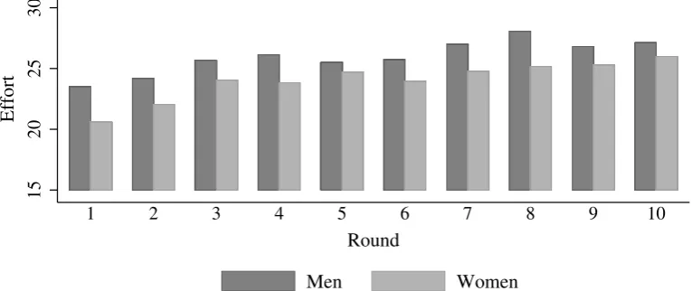
Figure 2 presents an initial summary of the raw data, split by gender. Effort choices range
from 0 to 41. Figure 2(a) shows that the distribution of effort choices for men has a bigger
right-hand tail than that for women, while Figure 2(b) shows that the effect persists during the
second half of the experiment.
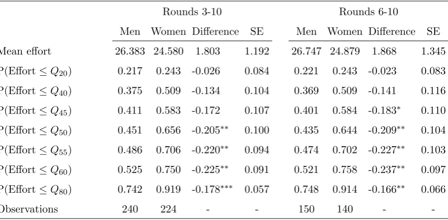
The left-hand panel of Table 1 validates these observations: the proportion of women in
the right-hand tail of the overall distribution of effort choices is significantly smaller than for
men. For example, 75% of women’s work efforts lie at or below the 60th
percentile of the effort
2
In the practice rounds, the subjects were not told whether they had won or lost.
3
0
.02
.04
.06
.08
.1
Density
0 10 20 30 40
Effort
Men Women
kernel = epanechnikov, bandwidth = 1.7835
(a) Distributions of efforts for rounds 3-10.
0
.02
.04
.06
.08
.1
Density
0 10 20 30 40
Effort
Men Women
kernel = epanechnikov, bandwidth = 1.9593
[image:9.595.88.530.93.218.2](b) Distributions of efforts for rounds 6-10.
Figure 2: Distributions of effort choices.
distribution (the proportion is significantly greater than for men at the 5% level) and 92% lie at
or below the 80th
[image:9.595.77.528.380.602.2](significantly greater than for men at the 1% level). The right-hand panel of
Table 1 shows that these distributional differences are persistent, as suggested by Figure 2(b).
Rounds 3-10 Rounds 6-10
Men Women Difference SE Men Women Difference SE
Mean effort 26.383 24.580 1.803 1.192 26.747 24.879 1.868 1.345
P(Effort≤Q20) 0.217 0.243 -0.026 0.084 0.221 0.243 -0.023 0.083
P(Effort≤Q40) 0.375 0.509 -0.134 0.104 0.369 0.509 -0.141 0.116
P(Effort≤Q45) 0.411 0.583 -0.172 0.107 0.401 0.584 -0.183∗ 0.110
P(Effort≤Q50) 0.451 0.656 -0.205∗∗ 0.100 0.435 0.644 -0.209∗∗ 0.104
P(Effort≤Q55) 0.486 0.706 -0.220∗∗ 0.094 0.474 0.702 -0.227∗∗ 0.103
P(Effort≤Q60) 0.525 0.750 -0.225∗∗ 0.091 0.521 0.758 -0.237∗∗ 0.097
P(Effort≤Q80) 0.742 0.919 -0.178∗∗∗ 0.057 0.748 0.914 -0.166∗∗ 0.066
Observations 240 224 - - 150 140 -
-Note 1: ∗,∗∗and∗∗∗ denote, respectively, significance at the 10%, 5% and 1% levels (2-sided tests). Standard
errors are bootstrapped allowing clustering at the subject level.
Note 2: P(Effort≤Qj) denotes the proportion of observations at or below thej
th
percentile of the distribution of effort choices, pooled over men and women. Thejth percentile is defined as the smallest effort level such that j% or more of observations lie at or below this level: because effort is discrete, we can therefore have P(Effort≤Qj)> j%.
Table 1: Descriptive analysis of effort choices of men and women.
The tendency for women not to exert high levels of effort is so strong that 66% of women’s
work efforts lie at or below the median, and men complete 1.8 sliders more than women on
by gender: men complete more sliders on average in every round.4 Significance tests provide
support for this gender performance gap: Table 1 reports that the proportion of women’s work
efforts at or below the median is significantly greater than for men at the 5% level (for rounds
3 onwards and for rounds 6 onwards); and a likelihood-ratio test shows that, jointly, the means
and variances of the distributions of work effort split by gender are significantly different from
each other (rounds 3 onwards: p = 0.007; rounds 6 onwards: p= 0.027).5
However, the mean
performance difference of 1.8 sliders alone is not quite significant at conventional levels (as
outliers cause the variance to be high).
15
20
25
30
Effort
1 2 3 4 5 6 7 8 9 10
Round
[image:10.595.84.467.258.419.2]Men Women
Figure 3: Round by round mean effort choices.
4
Empirical analysis
What factors might help to explain the differences in work effort by gender outlined in Section 3?
Clearly, men and women may differ in average ability. In this paper, we focus on a further
explanation: men and women may respond differently to good and bad luck. In particular,
we look for gender differences in how Second Movers respond to whether they won or lost the
previous two rounds of competition.6
We first outline our model of behavior and discuss the
estimation strategy, and then report the results of the analysis.
4
The gender difference in mean effort might change over rounds due to differences in learning by gender and due to differential responses to winning and losing in earlier rounds. Our empirical model includes both effects.
5
This likelihood ratio test assumes that effort is the sum of a deterministic component and normally distributed transient and permanent unobserved heterogeneity. The unrestricted likelihood allows the mean of effort, and also the standard deviations of both the permanent and transitory unobservables, to vary by gender.
6
4.1 Model and estimation strategy
We model behavior for rounds 3 onwards to allow for the effect on productivity of winning
or losing in the two preceding rounds. Our econometric strategy additionally accounts for
permanent individual-level ability differences, time effects and prize effects. Specifically, for
males, work effort in the rth
round for the nth
Second Mover,en,r, is given by
en,r =
2
∑
j=1
(
βjMLn,r−j+γMj Wn,r−j ×vn,r−j+θjMLn,r−j ×vn,r−j )
+κMvn,r+δrM+µn+un,r, (1)
and for female Second Movers en,r is given by the same expression replacing eachM (for male)
with F (for female).
In (1)Ln,r−1 is a dummy variable which takes a value of 1 if the nth Second Mover lost in
the previous round and zero otherwise. Wn,r−1 is the equivalent dummy variable in the case
of a win. Ln,r−2 and Wn,r−2 are dummy variables for losing and winning two rounds previous
to round r. Given the method of determining the allocation of each pair’s prize in each round
described above in Section 2, the values of these dummy variables depend partly on the relative
work effort of the pair members, and partly on luck, in the form of the random draw.
vn,r represents the prize that thenth Second Mover was competing for in therth round. We
interact the dummy variables for winning and losing with the relevant prizes to allow for the
fact that the impact of winning or losing might depend on how much was won or on how much
could have been won. We also include dummy variables for losing without a prize interaction to
determine the impact of losing rather than winning independent of the prize.7
The inclusion of theκM andκF terms controls for any effect of the current prize on behavior.
δMr and δrF are round specific intercepts, which control for differential learning and average
ability by gender. µn is a round invariant subject-specific fixed effect, which allows for residual
heterogeneity in ability across subjects that is not picked up by the gender and round specific
intercepts. Lastly, un,r is an unobservable that varies over rounds and over Second Movers and
captures differences between rounds in a Second Mover’s effort choice that cannot be attributed
to the other terms in the model. un,r is assumed to have mean zero and to be uncorrelated over
individuals.
The above constitutes a dynamic linear panel data model. By construction, the fixed effect
µnimpacts on previous efforts, and therefore on previous winning and losing (as individuals with
high effort in an earlier round are more likely to have won the prize in that round), and also affects
current effort. Hence, the error term (µn+un,r) is correlated with previous winning and losing,
7
and it follows that the OLS estimates of the parameters in (1) will be inconsistent. We obtain
consistent parameter estimates by using panel data Generalized Method of Moments techniques
(see Arellano and Bond, 1991 and Holtz-Eakin et al., 1988, and also Bossaerts et al., 2007, for an
application of Generalized Method of Moments in an experimental setting). Specifically, taking
first differences of (1) gives
∆en,r =
2
∑
j=1
(
βMj ∆Ln,r−j+γjM∆ (Wn,r−j×vn,r−j) +θMj ∆ (Ln,r−j×vn,r−j) )
+
κM∆vn,r+ ∆δMr + ∆un,r, for r = 4, ...,10, (2)
and an analogous equation can be written for females. First differencing therefore eliminates
the subject-specific fixed effects. However, a further endogeneity problem arises in the first
differenced equations because the transformed error term ∆un,r is correlated with the dummy
variables for winning or losing in roundr−1 (due to the correlation between un,r−1 and en,r−1
and therefore between un,r−1 and winning and losing in the previous round).
Similarly to Ham et al. (2005), we exploit randomization induced by the experimental design
to obtain a number of valid instruments for the variables measuring the previous competitive
outcomes in the first differenced equations: first, we use the random draws which determine
whether the nth Second Mover won the prize in the three rounds prior to roundr; second, we
use the random prizes in these earlier rounds; third we use the random draw interacted with the
random prize for each of these earlier rounds; and fourth we use the effort choice of thenthSecond Mover’s rival in these earlier rounds. Furthermore, we use the nth Second Mover’s own effort two and three rounds prior to round r, which under the assumption of zero serial correlation in
un,r are valid instruments (see footnote 12 for evidence supporting the assumption that un,r is
serially uncorrelated). All these instruments are also interacted with a dummy variable for the
subject being male.8
Appendix A shows that our results are robust to dropping various subsets
of these instruments.9
8
To limit instrument proliferation, we collapse the instrument set by applying each instrument to all available rounds jointly. Although competitive outcomes datedr−2 are not endogenous with respect to the first difference of the transitory errors, we instrument for these variables in the same way as for competitive outcomes dated
r−1 in order to maintain consistency. Our results are robust to this method of identifying the coefficients on competitive outcomes datedr−2. We identify the gender-specific current prize effects and the round-by-round changes in the gender-specific intercepts using standard orthogonality conditions based on the first differenced errors and the current prize and round dummies, and interactions of these variables with gender. Finally, we form two moment conditions based on the level equations for men and women, and these moments allow us to identify the level of the gender-specific intercepts.
9
4.2 Description of results
We start by reporting our parameter estimates and the associated behavioral effects. We then
consider whether our results can explain part of the gender difference in work efforts described
in Section 3.
4.2.1 Parameter estimates
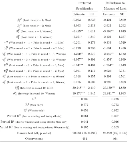
Table 2 presents the estimated parameters for our preferred specification (that is the model
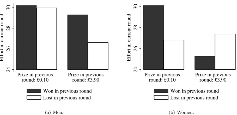
outlined in Section 4.1). Figure 4 shows how these parameter estimates translate into behavioral
effects of the competitive outcome in the preceding round on current effort provision.
The large negative estimate of β1F, which is significantly different from zero (2-sided p =
0.030), indicates a strong negative impact on current work effort for a woman of having lost in
the previous round independent of the value of the prize that she failed to win. However, we
find no such effect for men (βM
1 is close to zero and not significant). Reflecting the estimate
of βF
1, the difference between the first two bars of Figure 4(b) shows that for women having
experienced a loss in the previous round at the smallest prize of £0.10 instead of winning the
same prize of £0.10 induces a reduction in current work effort of 3.4 sliders. The magnitude of
this effect is sizeable in the context of a mean level of effort of 25.5 sliders in rounds 3 to 10.
In contrast, reflecting that the estimate of β1M is close to zero, the negligible difference between
the first two bars of Figure 4(a) shows that the current work effort of men does not respond
to the outcome of the previous round of competition when the prize in the previous round was
minimal. The estimates of βF
1 and β1M differ significantly (2-sided p = 0.061 in the preferred
specification; 2-sided p= 0.011 in specification R4 in Appendix A, which additionally controls
for the effects of competitive outcomes three rounds previously10
), which implies a significant
difference in how men and women respond to losing independent of the value of the prize that
they failed to win.
10
Preferred Robustness to
Specification Measure of Luck
Estimate SE Estimate SE
βM
1 (Lost roundr−1; Men) -0.093 0.836 -0.424 0.809
βM
2 (Lost roundr−2; Men) -3.093 2.213 -2.922 2.262
βF
1 (Lost roundr−1; Women) -3.499∗∗ 1.611 -3.169∗∗ 1.613
βF
2 (Lost roundr−2; Women) -2.271∗ 1.340 -2.121 1.367
γM1 (Won roundr−1×Prize in roundr−1; Men) -0.201 0.273 -0.333 0.529
γM2 (Won roundr−2×Prize in roundr−2; Men) -0.773 0.733 -1.584 1.456
γ1F (Won roundr−1×Prize in roundr−1; Women) -1.299∗∗ 0.570 -2.259∗∗ 1.132
γ2F (Won roundr−2×Prize in roundr−2; Women) -1.057∗∗ 0.491 -1.854∗ 0.999
θM
1 (Lost roundr−1×Prize in roundr−1; Men) -0.847∗∗ 0.431 -1.254∗∗ 0.549
θM
2 (Lost roundr−2×Prize in roundr−2; Men) 0.071 0.417 -0.025 0.731
θF
1 (Lost roundr−1×Prize in roundr−1; Women) 0.168 0.257 0.294 0.501
θF
2 (Lost roundr−2×Prize in roundr−2; Women) 0.125 0.502 0.292 0.988
δ10M (Intercept in round 10; Men) 30.248∗∗∗ 2.110 30.139∗∗∗ 1.880
δ10F (Intercept in round 10; Women) 30.370∗∗∗ 1.945 29.811∗∗∗ 1.993
R2
0.739 0.738
R2
(Men only) 0.772 0.773
R2
(Women only) 0.654 0.652
Partial R2
(due to winning and losing effects) 0.061 0.057
Partial R2
(due to winning and losing effects; Men only) 0.041 0.036
Partial R2
(due to winning and losing effects; Women only) 0.105 0.103
Hansen test (df, p value) 20.681 (16, 0.191) 23.299 (16, 0.106)
Observations 464 464
Note 1: ∗,∗∗ and∗∗∗denote, respectively, significance at the 10%, 5% and 1% levels (2-sided tests). Standard
errors are robust to heteroskedasticity and allow clustering at the subject level.
Note 2: The estimates of the contemporaneous prize effects (κM andκF) and of the intercepts (δM
r andδrF)
for rounds 3 to 9 are not reported in the table. The prize effects do not differ significantly by gender. Note 3: We show robustness to our measure of luck by re-estimating the model with the measures of previous
monetary winnings and losses expressed relative to expectations, rather than in absolute terms. LettingPn,r−j
represent, in proportionate terms, thenth Second Mover’s probability of winning the prize in roundr−j, the robustness to the measure of luck replacesγM
j Wn,r−j×vn,r−j withγMj Wn,r−j×vn,r−j×(1−Pn,r−j) and
θM
j Ln,r−j×vn,r−jwithθjMLn,r−j×vn,r−j×Pn,r−jfor males, and similarly for females. Because, on average,
[image:14.595.78.524.74.581.2]Pn,r−j= 0.5 the coefficients in this alternative specification tend to be higher.
24
26
28
30
Effort in current round
Prize in previous round: £0.10
Prize in previous round: £3.90 Won in previous round Lost in previous round
(a) Men.
24
26
28
30
Effort in current round
Prize in previous round: £0.10
Prize in previous round: £3.90 Won in previous round Lost in previous round
(b) Women.
Notes: The effects are presented for the average male and the average female in round 10, ignoring the contemporaneous prize effect and the impact of winning and losing two rounds previously (by setting
κM = βM
2 = γM2 = θ2M = 0 for males, and similarly for females). Thus, after winning the effort for men is
given byγM
1 ×v+δ10M and after losing it is given byβ1M +θM1 ×v+δM10, and similarly for females. Alternative
[image:15.595.85.540.73.295.2]assumptions would shift the bars for men up or down relative to those for women.
Figure 4: Graphical description of impact of winning or losing in previous round.
Our estimate ofθF
1 is close to zero and not significant, indicating that conditional on losing in
the previous round a woman’s current work effort does not depend on the value of the prize that
she failed to win. Graphically, this feature of our results is represented by the approximately
equal heights of the two white bars in Figure 4(b), which show women’s work effort following a
loss at prizes of £0.10 and£3.90 respectively.11
In contrast, our estimate ofθ1M is negative and
significantly different from zero (2-sided p = 0.049), implying that conditional on losing in the
previous round a man’s work effort decreases in the size of the prize that he failed to win. This
behavioral effect is illustrated in Figure 4(a) by the notably lower height of the white bar at a
prize of£3.90 as compared to the white bar at a prize of£0.10: after losing at a prize of£3.90 in
the previous round, the current work effort of men is 3.2 sliders lower than male work effort after
losing at a prize of £0.10. The estimates of θF
1 and θM1 differ significantly (2-sided p= 0.043;
2-sided p= 0.011 in specification R4 in Appendix A, which additionally controls for the effects
of competitive outcomes three rounds previously), which implies a significant difference in how
the responses of men and women to losing in the previous round depend on the value of the
prize that they failed to win.
The negative estimate of γ1F, which is significantly different from zero (2-sided p = 0.023),
indicates that conditional on winning in the previous round a woman’s current work effort
decreases in the size of the prize that she won. This is represented graphically in Figure 4(b)
11
by the lower height of the dark bar at a prize of £3.90 as compared to the dark bar at a
prize of £0.10: after winning a prize of £3.90 in the previous round, the current work effort
of women is about 4.9 sliders lower than after winning a prize of £0.10. For a man, however,
conditional on winning in the previous round the value of the prize that he won does not impact
on current behavior (γ1M is close to zero and insignificant). This is illustrated graphically by
the approximately equal heights of the two dark bars in Figure 4(a). The estimates of γF
1 and
γM
1 differ significantly (2-sided p= 0.082; 2-sidedp= 0.081 in specification R4 in Appendix A,
which additionally controls for the effects of competitive outcomes three rounds previously),
which implies a significant difference in how the responses of men and women to winning in the
previous round depend on the value of the prize that they won.
The above results reveal some striking gender differences in behavioral responses to previous
competitive outcomes. In summary, the β1 and θ1 estimates together imply that, relative to
winning the smallest prize of£0.10, for women losing per se is detrimental to productivity, but
for men a loss impacts negatively on productivity only when the prize at stake is big enough.
Furthermore theγ1 estimates imply that, conditional on winning in the previous round, women’s
current work effort declines in the value of the prize, while there is no such effect for men.
Additionally, we note here that a χ2 test gives p = 0.052 for the joint null that β
1, θ1 and γ1
do not vary by gender (the corresponding pvalue based on specification R4 which additionally
controls for the effects of competitive outcomes three rounds previously is 0.039).
Table 2 also provides some evidence of the persistence of these effects for women. Losing
two rounds previously dampens current effort significantly (negative estimate of β2F; 2-sided
p= 0.090). The effect of the prize conditional on winning also persists for two rounds (negative
estimate of γF
2 ; 2-sided p = 0.031). In contrast, Table 2 shows that we find no evidence of
persistence for men over a two-round horizon. A χ2
test gives p= 0.458 for the joint null that
β2,θ2andγ2do not vary by gender, and therefore overall we cannot show any significant gender
differences in the effects of competitive outcomes two rounds previously on current behavior.
Finally, as outlined in Appendix A, we find no evidence that winning or losing has any impact
on behavior three rounds later, either for men or for women.
The partial R2 shows that about 6% of the variation across subjects and rounds observed in the data can be attributed to the winning and losing terms in our model. For women, the
partial R2
suggests that about 11% of the variation can be attributed to the luck terms, while
for men about 4% of the variation can be attributed to the response to luck. The Hansen test
additional moments.12
In the preferred specification, we use winning and losing as our measure of luck. Arguably, a
winner is luckier the more she wins relative to what she expected to win in the round, which in
turn depends both on the prize and her probability of winning (from the experimental design,
this probability depends linearly on the difference between the winner’s effort choice and that of
her rival). Similarly a loser is more unlucky the more she expected to win. In order to explore
the robustness of our results to the measure of luck we re-estimate the model replacing previous
winnings and losses with the value of previous winnings and losses relative to expectations.
Note 3 in Table 2 provides further details. The second column of Table 2 shows that working
instead with this purer measure of luck does not materially affect our results.13
The reason
is that there is little variation in winning probabilities across winners or across losers, because
winning probabilities are mostly condensed in the range [40%,60%]. For winners, 79.2% of
observations lie in this range across all 10 rounds, while 80.8% do for losers.
4.2.2 Luck and gender differences in efforts
Section 3 described how the whole distribution of work efforts are different by gender, with men
exhibiting a higher average level of effort. On average, men completed about 1.8 sliders more
than women, and a significantly greater proportion of women’s work efforts lie below the sample
median. We now use a decomposition analysis to determine the extent to which the differential
responses to winning and losing by gender described above can account for this performance
gap between men and women.
The decomposition analysis sets the coefficients on the winning and losing terms to zero, while
continuing to use the other parameter estimates. To undertake this exercise, we also make the
normalizing assumption that winning the smallest prize of£0.10 has the same behavioral impact
on men and women, so that none of the gender performance gap after winning the smallest prize
is due to a differential response to previous competitive outcomes.14
Under this assumption,
and with the coefficients on the winning and losing terms set to zero, the decomposition analysis
predicts that men outperform women by about 0.9 sliders. Thus the differential responses to
previous competitive outcomes explain the rest of the performance gap observed in rounds 3 to
10, and so approximately 50% of the performance gap is due to the winning and losing effects.
12
In order to test for zero serial correlation inun,r, we run an Arellano-Bond test for the null hypothesis of
zero second order autocorrelation in ∆un,r. This givespvalues of 0.202 for the preferred specification and 0.143
for the specification used to check robustness to our measure of luck.
13
The main difference is that in this alternative specification the evidence for the persistence of the effects for women is weaker.
14
5
Discussion & conclusion
To the best of our knowledge our paper is the first to study how the productivity of men and
women responds to the outcome of previous competitions. Labor markets tend to exhibit
re-peated competitive interactions: for instance, career opportunities often involve multiple rounds
of competition for new positions, promotions, bonuses and pay rises. Our novel findings may
help in understanding better some of the sources and dynamics of gender differences in such
com-petitive environments. Alongside more traditional explanations such as discrimination, ability
differences and a stronger preference for investing in child-rearing, our findings suggest that the
gender gap in labor markets may be driven partly by actual and anticipated responses to the
process of winning and losing during competition.
In particular, differential responses by gender to wining and losing account for a significant
portion of the gender performance gap that we observe in our experiment: to the extent that
these differential responses are also important outside of the experimental laboratory, women in
actual labor markets will perform relatively worse as compared to men when forced to compete.
Furthermore, if the differential responses to winning and losing that we find are anticipated,
women may choose to select into competitive environments at a lower rate than men do. Our
results in a dynamic context thus suggest a new mechanism which may help to explain the
find-ings of Niederle and Vesterlund (2007) and others that women shy away from competition even
after allowing for differential levels of confidence, risk aversion and aversion to feedback about
relative performance. As yet, beyond informal appeals to evolutionary theory, no convincing
mechanism or explanation for this residual dislike for competition has been found. As Gneezy
et al. (2009) put it: “An important puzzle in this literature relates to the underlying factors
responsible for the observed differences in competitive inclinations” (p. 1637).
Further research is required to pin down the processes and mechanisms that might underlie
and drive the differential responses by gender to winning and losing that we have identified.
Whether these differences are mainly driven by nature or by environmental factors will determine
appropriate labor market policy responses. One hypothesis is that winning and losing induce
psycho-physiological responses which affect behavior in the next round and which vary by gender.
The psycho-physiology literature has identified differences across gender in how mood (Mazur
et al., 1997), blood pressure (Holt-Lunstad et al., 2001) and confidence (Roberts, 1991) respond
to competitive outcomes. There is evidence that, compared to men, women suffer greater anxiety
and elevated cortisol when they compete (Filaire et al., 2009).15
Buser (2009) and Wozniak et al.
(2010) link competition aversion to sex hormones, which also suggests that physiology might
15
be important. On the other hand, Booth and Nolen (2009) and Gneezy et al. (2009) link
competition aversion to educational and familial environments, which suggests that factors such
as upbringing, culture and institutions could also play a significant role in how men and women
react to success and failure in competitive environments.
Further research could also help explain the negative response in work effort after winning a
large prize as compared to work effort after winning a small prize that we find for women, which
may be related to guilt or egalitarianism. The psychological discomfort associated with guilt
may impact directly on performance. Alternatively, if women feel that winning a large prize
was undeserved they may wish to reduce effort in the next period to reduce their probability
of winning and so redistribute wealth in expectation to other members of the subject pool (see
Grund and Sliwka, 2005, and Gill and Stone, 2010, for analyses of how, respectively, inequity and
desert concerns affect competitive behavior). A number of studies provide evidence from dictator
games that women are more inequity averse or egalitarian than men (e.g., Eckel and Grossman,
1998, and Andreoni and Vesterlund, 2001; see Croson and Gneezy, 2009, for a survey of the
evidence). Interestingly, Bartling et al. (2009) find that the vast majority of their all-female
sample are ‘aheadness-averse’, that is they are averse to favorable inequity; furthermore, the
study finds a significant negative effect of aheadness-aversion on the choice to enter a tournament
for women, but no similar effect of aversion to unfavorable inequity.
Finally, we encourage researchers to uncover evidence of how men and women respond to
previous competitive outcomes in the field. Our laboratory environment and experimental
de-sign allow us sufficient control to identify cleanly responses to winning and losing. Nonetheless,
complementary evidence of the importance of the effects that we find from labor markets,
ed-ucational environments and public elections where competition plays a large role and gender
differences in outcomes are apparent would be invaluable. Wozniak (forthcoming) provides an
interesting first foray in this direction by looking at the degree to which winning is positively
Appendix
A
Robustness
We examine the robustness of our results by: (i) re-estimating the model using different, more
restrictive, instrument sets and (ii) estimating the parameters of a model specification that
additionally includes variables describing competitive outcomes three rounds previously.
Results R1, R2 and R3 in Table 3 show that the parameter estimates of the preferred
specification in Table 2 are substantively unaffected by various restrictions on the instrument
set, which are detailed in the notes to Table 3. The fourth set of results in Table 3, labeled R4,
shows that there are no effects on work effort in a given round of competitive outcomes three
rounds previously, and that the parameter estimates in Table 2 are not materially affected by
the inclusion of the variables detailing these extra competitive outcomes.
B
Experimental instructions
Please open the brown envelope you have just collected. I am reading from the four page
instructions sheet which you will find in your brown envelope. [Open brown envelope]
Thank you for participating in this session. There will be a number of pauses for you to ask
questions. During such a pause, please raise your hand if you want to ask a question. Apart
from asking questions in this way, you must not communicate with anybody in this room. Please
now turn off mobile phones and any other electronic devices. These must remain turned off for
the duration of this session. Are there any questions?
You have been allocated to a computer booth according to the number on the card you
selected as you came in. You must not look into any of the other computer booths at any time
during this session. As you came in you also selected a white sealed envelope. Please now open
your white envelope. [Open white envelope]
Each white envelope contains a different four digit Participant ID number. To ensure
anonymity, your actions in this session are linked to this Participant ID number and at the
end of this session you will be paid by Participant ID number. You will be paid a show up fee
of £4 together with any money you accumulate during this session. The amount of money you
accumulate will depend partly on your actions, partly on the actions of others and partly on
chance. All payments will be made in cash in another room. Neither I nor any of the other
participants will see how much you have been paid. Please follow the instructions that will
appear shortly on your computer screen to enter your four digit Participant ID number. [Enter
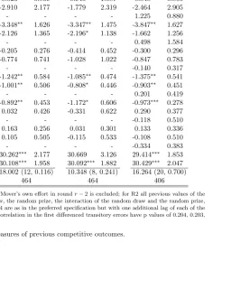
R1 R2 R3 R4
Estimate SE Estimate SE Estimate SE Estimate SE
β1M (Lost roundr−1; Men) -0.180 0.828 -0.023 0.869 0.940 1.087 0.848 0.866
βM
2 (Lost roundr−2; Men) -3.206 2.281 -2.910 2.177 -1.779 2.319 -2.464 2.905
β3M (Lost roundr−3; Men) - - - 1.225 0.880
β1F (Lost roundr−1; Women) -3.417∗∗ 1.633 -3.348∗∗ 1.626 -3.347∗∗ 1.475 -3.847∗∗ 1.627
βF
2 (Lost roundr−2; Women) -2.209 1.355 -2.126 1.365 -2.196∗ 1.138 -1.662 1.256
βF
3 (Lost roundr−3; Women) - - - 0.498 1.584
γM1 (Won roundr−1×Prize in roundr−1; Men) -0.226 0.277 -0.205 0.276 -0.414 0.452 -0.300 0.296
γM
2 (Won roundr−2×Prize in roundr−2; Men) -0.821 0.758 -0.774 0.741 -1.028 1.022 -0.847 0.783
γM
3 (Won roundr−3×Prize in roundr−3; Men) - - - -0.140 0.317
γ1F (Won roundr−1×Prize in roundr−1; Women) -1.270∗∗ 0.583 -1.242∗∗ 0.584 -1.085∗∗ 0.474 -1.375∗∗ 0.541
γF
2 (Won roundr−2×Prize in roundr−2; Women) -1.021∗∗ 0.506 -1.001∗∗ 0.506 -0.808∗ 0.446 -0.903∗∗ 0.451
γF
3 (Won roundr−3×Prize in roundr−3; Women) - - - 0.201 0.419
θM1 (Lost roundr−1×Prize in roundr−1; Men) -0.876∗∗ 0.445 -0.892∗∗ 0.453 -1.172∗ 0.606 -0.973∗∗∗ 0.278
θM
2 (Lost roundr−2×Prize in roundr−2; Men) 0.053 0.424 0.032 0.426 -0.331 0.622 0.290 0.377
θM
3 (Lost roundr−3×Prize in roundr−3; Men) - - - -0.118 0.510
θ1F (Lost roundr−1×Prize in roundr−1; Women) 0.166 0.257 0.163 0.256 0.031 0.301 0.133 0.336
θF
2 (Lost roundr−2×Prize in roundr−2; Women) 0.116 0.504 0.105 0.505 -0.115 0.533 -0.108 0.510
θF
3 (Lost roundr−3×Prize in roundr−3; Women) - - - -0.334 0.383
δ10M (Intercept in round 10; Men) 30.479∗∗∗ 2.216 30.262∗∗∗ 2.177 30.669 3.126 29.414∗∗∗ 1.853
δF
10(Intercept in round 10; Women) 30.229∗∗∗ 1.978 30.108∗∗∗ 1.958 30.092∗∗∗ 1.882 30.429∗∗∗ 2.047
Hansen test (df, p value) 19.590 (14, 0.144) 18.002 (12, 0.116) 10.348 (8, 0.241) 16.264 (20, 0.700)
Observations 464 464 464 406
Notes: For R1 the instrument set is as in the preferred specification, except that the Second Mover’s own effort in round r−2 is excluded; for R2 all previous values of the
[image:21.595.318.743.90.421.2]Second Mover’s own effort are excluded; and for R3 the most recent value of the random draw, the random prize, the interaction of the random draw and the random prize, and the effort of the Second Mover’s rival are excluded. Instruments used to obtain results R4 are as in the preferred specification but with one additional lag of each of the instrumental variables. Arellano-Bond tests for the null hypothesis of zero second order autocorrelation in the first differenced transitory errors have p values of 0.204, 0.203, 0.297 and 0.170 for R1-R4 respectively. See also notes 1 and 2 in Table 2.
Table 3: Robustness to choice of instruments and measures of previous competitive outcomes.
envelope, and keep this safe as your Participant ID number will be required for payment at the
end.
This session consists of 2 practice rounds, for which you will not be paid, followed by 10
paying rounds with money prizes. In each round you will undertake an identical task lasting
120 seconds. The task will consist of a screen with 48 sliders. Each slider is initially positioned
at 0 and can be moved as far as 100. Each slider has a number to its right showing its current
position. You can use the mouse in any way you like to move each slider. You can readjust
the position of each slider as many times as you wish. Your “points score” in the task will be
the number of sliders positioned at exactly 50 at the end of the 120 seconds. Are there any
questions?
Before the first practice round, you will discover whether you are a “First Mover” or a
“Second Mover”. You will remain either a First Mover or a Second Mover for the entirety of
this session.
In each round, you will be paired. One pair member will be a First Mover and the other
will be a Second Mover. The First Mover will undertake the task first, and then the Second
Mover will undertake the task. The Second Mover will see the First Mover’s points score before
starting the task.
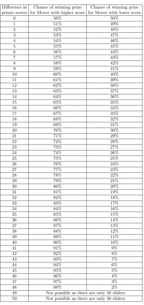
In each paying round, there will be a prize which one pair member will win. Each pair’s
prize will be chosen randomly at the beginning of the round and will be between £0.10 and
£3.90. The winner of the prize will depend on the difference between the First Mover’s and the
Second Mover’s points scores and some element of chance. If the points scores are the same,
each pair member will have a 50% chance of winning the prize. If the points scores are not the
same, the chance of winning for the pair member with the higher points score increases by 1
percentage point for every increase of 1 in the difference between the points scores, while the
chance of winning for the pair member with the lower points score correspondingly decreases
by 1 percentage point. The table at the end of these instructions gives the chance of winning
for any points score difference. Please look at this table now. [Look at table] Are there any
questions?
During each task, a number of pieces of information will appear at the top of your screen,
including the time remaining, the round number, whether you are a First Mover or a Second
Mover, the prize for the round and your points score in the task so far. If you are a Second
Mover, you will also see the points score of the First Mover you are paired with.
After both pair members have completed the task, each pair member will see a summary
screen showing their own points score, the other pair member’s points score, their probability
We will now start the first of the two practice rounds. In the practice rounds, you will be
paired with an automaton who behaves randomly. Before we start, are there any questions?
Please look at your screen now. [First practice round] Before we start the second practice
round, are there any questions? Please look at your screen now. [Second practice round]
Are there any questions?
The practice rounds are finished. We will now move on to the 10 paying rounds. In every
paying round, each First Mover will be paired with a Second Mover. The pairings will be changed
after every round and pairings will not depend on your previous actions. You will not be paired
with the same person twice. Furthermore, the pairings are done in such a way that the actions
you take in one round cannot affect the actions of the people you will be paired with in later
rounds. This also means that the actions of the person you are paired with in a given round
cannot be affected by your actions in earlier rounds. (If you are interested, this is because you
will not be paired with a person who was paired with someone who had been paired with you,
and you will not be paired with a person who was paired with someone who had been paired
with someone who had been paired with you, and so on.) Are there any questions?
We will now start the 10 paying rounds. There will be no pauses between the rounds.
Before we start the paying rounds, are there any remaining questions? There will be no further
opportunities to ask questions. Please look at your screen now. [10 paying rounds]
The session is now complete. Your total cash payment, including the show up fee, is displayed
on your screen. Please leave the room one by one when asked to do so to receive your payment.
Remember to bring the envelope containing your four digit Participant ID number with you but
Difference in Chance of winning prize Chance of winning prize points scores for Mover with higher score for Mover with lower score
0 50% 50%
1 51% 49%
2 52% 48%
3 53% 47%
4 54% 46%
5 55% 45%
6 56% 44%
7 57% 43%
8 58% 42%
9 59% 41%
10 60% 40%
11 61% 39%
12 62% 38%
13 63% 37%
14 64% 36%
15 65% 35%
16 66% 34%
17 67% 33%
18 68% 32%
19 69% 31%
20 70% 30%
21 71% 29%
22 72% 28%
23 73% 27%
24 74% 26%
25 75% 25%
26 76% 24%
27 77% 23%
28 78% 22%
29 79% 21%
30 80% 20%
31 81% 19%
32 82% 18%
33 83% 17%
34 84% 16%
35 85% 15%
36 86% 14%
37 87% 13%
38 88% 12%
39 89% 11%
40 90% 10%
41 91% 9%
42 92% 8%
43 93% 7%
44 94% 6%
45 95% 5%
46 96% 4%
47 97% 3%
48 98% 2%
[image:24.595.153.445.98.716.2]49 Not possible as there are only 48 sliders 50 Not possible as there are only 48 sliders
References
Altonji, J.G. and Blank, R.M. (1999). Race and gender in the labor market. In Handbook of Labor Economics, Vol. 3, ed. Orley Ashenfelter and David Card, 3143–3259. Amsterdam: North Holland
Andreoni, J.andVesterlund, L.(2001). Which is the fair sex? Gender differences in altruism.
Quarterly Journal of Economics, 116(1): 293–312
Arellano, M. and Bond, S. (1991). Some tests of specification for panel data. Review of Economic Studies, 58(2): 277–297
Bartling, B., Fehr, E., Mar´echal, M.A., and Schunk, D. (2009). Egalitarianism and competitiveness. American Economic Review: Papers and Proceedings, 99(2): 93–98
Bertrand, M. and Hallock, K.F. (2001). The gender gap in top corporate jobs. Industrial and Labor Relations Review, 55(1): 3–21
Bognanno, M.L.(2001). Corporate tournaments.Journal of Labor Economics, 19(2): 290–315
Booth, A.L. andNolen, P.J.(2009). Choosing to compete: How different are girls and boys?
IZA, Discussion Paper 4027
Bossaerts, P.,Plott, C., and Zame, W.R. (2007). Prices and portfolio choices in financial markets: Theory, econometrics, experiments. Econometrica, 75(4): 993–1038
Buser, T.(2009). The impact of female sex hormones on competitiveness. Tinbergen Institute, Discussion Paper 2009-082/3
Cason, T.N.,Masters, W.A., andSheremeta, R.M.(2010). Entry into winner-take-all and proportional-prize contests: An experimental study. Journal of Public Economics, 94(9-10): 604–611
Charness, G. and Kuhn, P. (2010). Lab labor: What can labor economists learn from the lab? InHandbook of Labor Economics, Vol. 4, ed. Orley Ashenfelter and David Card, 229-330. Amsterdam: North Holland
Charness, G. andVilleval, M.C.(2009). Cooperation and Competition in Intergenerational Experiments in the Field and the Laboratory. American Economic Review, 99(3): 956–978
Cooper, R., DeJong, D.V., Forsythe, R., and Ross, T.W.(1996). Cooperation without reputation: Experimental evidence from prisoner’s dilemma games. Games and Economic Behavior, 12(2): 187–218
Croson, R. and Gneezy, U. (2009). Gender differences in preferences. Journal of Economic Literature, 47(2): 448–474
Eckel, C.C. (2008). The gender gap: Using the lab as a window on the market. Frontiers in the Economics of Gender. Siena Studies in Political Economy. Routledge, London, 223–242
Eckel, C.C. and Grossman, P.J.(1998). Are women less selfish than men?: Evidence from dictator experiments. Economic Journal, 108(448): 726–735
Eriksson, T. (1999). Executive compensation and tournament theory: Empirical tests on Danish data. Journal of Labor Economics, 17(2): 262–280
Filaire, E., Alix, D., Ferrand, C., and Verger, M. (2009). Psychophysiological stress in tennis players during the first single match of a tournament.Psychoneuroendocrinology, 34(1): 150–157
Fischbacher, U.(2007). z-Tree: Zurich toolbox for ready-made economic experiments. Exper-imental Economics, 10(2): 171–178
Fletschner, D.,Anderson, C., andCullen, A.(2010). Are women as likely to take risks and compete? behavioural findings from central vietnam. The Journal of Development Studies, 46(8): 1459–1479
Gill, D. and Prowse, V. (2010). Gender differences and dynamics in competition: The role of luck. IZA Discussion Paper 5022
Gill, D. andProwse, V.(forthcoming). A structural analysis of disappointment aversion in a real effort competition. American Economic Review
Gill, D. and Stone, R. (2010). Fairness and desert in tournaments. Games and Economic Behavior, 69(2): 346–364
Gneezy, U., Leonard, K.L., and List, J.A. (2009). Gender differences in competition: Evidence from a matrilineal and a patriarchal society. Econometrica, 77(5): 1637–1664
Gneezy, U.,Niederle, M., andRustichini, A.(2003). Performance in competitive environ-ments: Gender differences. Quarterly Journal of Economics, 118(3): 1049–1074
Gneezy, U. and Rustichini, A. (2004). Gender and competition at a young age. American Economic Review: Papers and Proceedings, 94(2): 377–381
Grund, C.andSliwka, D.(2005). Envy and compassion in tournaments.Journal of Economics and Management Strategy, 14(1): 187–207
Gupta, N.D.,Poulsen, A., andVilleval, M.C.(2005). Male and female competitive behav-ior: Experimental evidence. IZA, Discussion Paper 1833
Ham, J.C.,Kagel, J.H., and Lehrer, S.F.(2005). Randomization, endogeneity and labora-tory experiments: The role of cash balances in private value auctions.Journal of Econometrics, 125(1-2): 175–205
Holt-Lunstad, J.,Clayton, C.J., and Uchino, B.N.(2001). Gender differences in cardio-vascular reactivity to competitive stress: The impact of gender of competitor and competition outcome. International Journal of Behavioral Medicine, 8(2): 91–102
Holtz-Eakin, D., Newey, W., and Rosen, H. (1988). Estimating vector autoregressions with panel data. Econometrica, 56(6): 1371–1395
Kamas, L.andPreston, A.(forthcoming). The importance of being confident: Gender, career choice, and willingness to compete. Journal of Economic Behavior and Organization
Kleinjans, K.J. (2009). Do gender differences in preferences for competition matter for occu-pational expectations? Journal of Economic Psychology, 30(5): 701–710
Lazear, E.P. and Rosen, S. (1981). Rank-order tournaments as optimum labor contracts.
Journal of Political Economy, 89(5): 841–864
Mazur, A.,Susman, E.J., andEdelbrock, S.(1997). Sex difference in testosterone response to a video game contest. Evolution and Human Behavior, 18(5): 317–326
Niederle, M., Segal, C., and Vesterlund, L. (2010). How costly is diversity? Affirmative action in light of gender differences in competitiveness. Stanford University, Mimeo
Niederle, M. and Vesterlund, L. (2007). Do women shy away from competition? Do men compete too much? Quarterly Journal of Economics, 122(3): 1067–1101
Ors, E.,Palomino, F., andPeyrache, E.(2008). Performance gender-gap: Does competition matter? CEPR, Discussion Paper 6891
Roberts, T.A.(1991). Gender and the influence of evaluations on self-assessments in achieve-ment settings. Psychological Bulletin, 109(2): 297–308
Vandegrift, D. and Yavas, A. (2009). Men, women, and competition: An experimental test of behavior. Journal of Economic Behavior and Organization, 72(1): 554–570
Wozniak, D.(forthcoming). Gender differences in a market with relative performance feedback: Professional tennis players. Journal of Economic Behavior and Organization
Wozniak, D., Harbaugh, W.T., and Mayr, U. (2010). Choices about competition: Dif-ferences by gender and hormonal fluctuations, and the role of relative performance feedback.