Munich Personal RePEc Archive
A Note on institutional hierarchy and
volatility in financial markets
Alfarano, Simone and Milakovic, Mishael and Raddant,
Matthias
Universitat Jaume I de Castellò
2011
Online at
https://mpra.ub.uni-muenchen.de/30902/
A Note on Institutional Hierarchy and Volatility in
Financial Markets
∗S. Alfaranoa
, M. Milakovi´c†b
, and M. Raddantc
a
Department of Economics, University Jaume I, Castell´on, Spain
b
Department of Economics, University of Bamberg, Germany
c
Institute for the World Economy (IfW), Kiel, Germany
May 10, 2011
Abstract
From a statistical point of view, the prevalence of non-Gaussian distributions in financial returns and their volatilities shows that the Central Limit Theorem (CLT) often does not apply in financial mar-kets. In this paper we take the position that the independence as-sumption of the CLT is violated by herding tendencies among market participants, and investigate whether a generic probabilistic herding model can reproduce non-Gaussian statistics in systems with a large number of agents. It is well-known that the presence of a herding mech-anism in the model is not sufficient for non-Gaussian properties, which crucially depend on the details of the communication network among agents. The main contribution of this paper is to show that certain hierarchical networks, which portray the institutional structure of fund investment, warrant non-Gaussian properties for any system size and even lead to an increase in system-wide volatility. Viewed from this perspective, the mere existence of financial institutions with socially interacting managers contributes considerably to financial volatility.
Keywords: Herding, financial volatility, networks, core-periphery.
JEL codes: G10, C46, D85, E19.
∗We gratefully acknowledge financial support by the Volkswagen Foundation through
their grant on “Complex Networks As Interdisciplinary Phenomena.” MM is thankful for financial support from theResearch Promotion Plan 2010 of Universitat Jaume I, received during his visit to Castell´on in that year. Comments by Albrecht Irle, Jonas Kauschke, Thomas Lux, and two anonymous referees are greatly appreciated.
1
Introduction
Financial time series exhibit ubiquitous non-Gaussian statistical regularities across different countries, assets, and time frequencies. The two most promi-nent features concern the fluctuations in the prices of financial assets, which exhibit heavy tails and clustered volatility (see, e.g., Cont, 2001; Pagan, 1996). From a statistical point of view, the prevalence of non-Gaussian dis-tributions in returns and their volatilities testifies to the importance of long-range correlations, which ultimately prevent the application of the Central Limit Theorem (CLT). Traditional finance has paid little, if any, attention to the origins of these statistical regularities and to the possibly most challeng-ing question implied by the violation of the CLT: how does a complex system like the financial market actually allow for a large scale coordination of the trading positions among millions of agents? The established literature on informational cascades (see, e.g., Banerjee, 1992; Bikhchandani et al., 1992; Chamley, 2004) does not address this question because it considers a static, sequential Bayesian updating approach with a constant ‘true’ state of the world and lacks any connection to the stylized facts of financial returns. The three major strands of the agent-based finance literature, on the other hand, argue in unison that it is precisely the perpetually alternating coordination of trading strategies over time that is responsible for the stylized facts of financial returns. Yet each of the approaches has to deal with its own set of problems.
the present paper, is inspired by entomological experiments concerning ants’ foraging behavior that Kirman (1991, 1993) utilized to propose a stochastic herding model of opinion formation among financial investors. These models endogenously create swings and herding behavior in aggregate expectations through social agent interaction, while the stationary distribution of the stochastic process of opinion formation describes thestatistical equilibrium
of the model.
The ‘ant model’ has been reasonably successful in replicating the sta-tistical features of financial returns, but Alfarano et al. (2008) have shown analytically that Kirman’s original model suffers from the problem of self-averaging or N-dependence:1
the model’s ability to replicate the stylized facts vanishes for a given parametrization when the system sizeN increases, a quite common feature in agent-based models that has received relatively minor attention so far (see, e.g., Aoki, 2008; Egenter et al., 1999; Lux and Schornstein, 2005). Alfarano and Milakovi´c (2009) establish a direct link be-tween N-(in)dependence and the communication network among agents in a generalized version of Kirman’s original model. They show that the model is immune to self-averaging if the relative communication range of agents remains unchanged under an enlargement of system size. Interestingly and rather counter-intuitively, other network features like the functional form of the degree distribution, the average clustering coefficient, the graph diame-ter, or the extent of assortative mixing have no impact on theN-dependence property. Put differently, the average number of neighbors per agent has to increase linearly with the total number of agentsN in order to overcome the problem of self-averaging in the generic herding model. Among prototypical network structures such as regular lattices, small-world, or scale-free net-works (see, e.g., Newman, 2003), it is only the random graph with constant linking probability that exhibits this feature, yet random graphs are hardly ever a realistic representation of socio-economic communication networks.
After all, the results of Alfarano et al. (2008) and Alfarano and Milakovi´c (2009) establish the model’s behavior when the number of agents tends to in-finity, at the same time illustrating that simple proto-typical network struc-tures (with the exception of the empirically unsatisfactory random graph) cannot overcome the problem of N-dependence. The present paper builds
1
Aoki utilizes the terms(non) self-averaging in lieu ofN-(in)dependence, and we will
on these insights and investigates whether a certain class of core-periphery networks might be capable of overcoming the self-averaging property of the original model. Here we consider a central network with bi-directional links betweencore agents oropinion leaders on one hand, and a relatively large number of uni-directionally linked followers in the periphery on the other. We vary the number of followers per core agent by randomly drawing from various distributions, and study the aggregate behavior of system-wide opin-ion dynamics under an increasing dispersopin-ion in the number of followers. In essence the hierarchical network corresponds to a weighted version of the original model. As we argue below, the weighted version is a reasonable first approximation of the institutional structure of financial fund investment. The central idea is that many investors effectively transfer control over in-vestment decisions to fund managers who in turn are socially interacting, with the opinions of some fund managers carrying greater weight than oth-ers, for instance because they manage larger funds or have performed more successfully in the past. It turns out that the analytical mean-field predic-tion used in Alfarano and Milakovi´c (2009) now significantly underestimates the volatility in system-wide opinion dynamics. The key implication of this result is that behavioral heterogeneity among interacting agents is not, as previously thought, the exclusive source of endogenously arising volatility in agent-based herding models, but that the hierarchical structure of fund investment is an important auxiliary source of financial volatility.
We take the position that investing in the presence of (actively managed) financial funds basically corresponds to the hierarchical core-periphery net-works we study here. Investors who are not wealthy enough to afford a broadly diversified portfolio of assets, those who participate in retirement plans, or those who simply feel that they lack the skills or time to make investment decisions often invest in some type or other of managed fund. Effectively such agents, who correspond to followers in the periphery of the network, transfer their wealth to the fund managers in the core, and ulti-mately allow those to make decisions for them. If fund managers socially interact with their peers, and empirical evidence by Hong et al. (2005) and Wermers (1999) strongly suggests that this is indeed the case, we arrive at the core-periphery networks that we study in this paper.
part of the network are amplified on a system-wide level. Therefore it seems rather ironic that investors who want to ‘play it safe’ by investing in a variety of managed funds will actually end up increasing system-wide volatility if they delegate investment decisions to herding-prone fund managers.
2
Generic Herding Model
In a prototypical interaction-based herding model of the Kirman type, the agent population of size N is divided into two groups, say, X and Y of sizes n and N −n, respectively. The time evolution of the group sizes is modeled as a Markov chain, characterized by a pair of transition rates that are sometimes also referred to as birth and death rates. Depending on the particular financial market framework, the two groups are typically labeled as fundamentalists and chartists, or optimists and pessimists, or buyers and sellers. The basic idea is that agents change state for personal reasons or under the influence of theneighbors with whom they socially interact during a given time period. The transition rate for an agentito switch from state
X to stateY in the Markov chain is
ω−i ≡ρi(X→Y) =ai+λi X
j6=i
DY(i, j), (1)
where ai governs the possibility of self-conversion due to idiosyncratic
fac-tors, e.g. the arrival of new information, while λi governs the interaction
strength between iand its neighbors. The function DY(i, j) is an indicator
function serving to count the number ofi’s neighbors that are in state Y,
DY(i, j) = (
1 if j is a Y-neighbor of i,
0 otherwise, (2)
hence the sum captures the (equally weighted) influence of the neighbors on agenti. Symmetrically, the transition rates in the opposite direction are given by
ω+
i ≡ρi(Y →X) =ai+λi
X
j6=i
DX(i, j). (3)
Leta=P
iai/N andλ=
P
iλi/N denote the averages of the behavioral
argument (see Alfarano and Milakovi´c, 2009) shows that the transition rates for a single switch on the aggregated system-wide level are
ω−=n
a+ λD
N (N −n)
, (4)
for a switch from X toY, and symmetrically
ω+= (N −n)
a+λD
N n
, (5)
for the reverse switch. An important result of the mean-field approach is that therelative communication range D/N ultimately determines whether the Markov chain is self-averaging or not. In the jargon of Alfarano et al. (2008), the non self-averaging case corresponds to “non-extensive” transition rates with a constant relative communication range, while the “extensive” transition rates, as in Kirman’s original model, lead to self-averaging and hence to counter-factual statistics of returns.2
Notice that non-extensive transition rates depend on the respective occupation numbers n and N − n, while extensive transition rates depend on the concentrations n/N and (N −n)/N of agents in the opposite state, and therefore on the average communication range per time period in the network. This apparently minor modification has a crucial impact on the aggregate properties of the herding model, as illustrated in Figure 1. Hence, in contrast to Kirman’s original model, the generalized transition rates (4) and (5) illustrate that network structure matters because the average number of neighbors explicitly enters the transition rates.
At any time, thestate of the systemrefers to the concentration of agents in one of the two states, say,z=n/N, which can be treated as a continuous variable for large N. None of the possible states of z ∈ [0,1] is an equi-librium in itself nor are there multiple equilibria in the orthodox economic sense. Equilibrium rather refers to the stationary distribution of the birth and death process (4) and (5). The distribution, that is the statistical equi-librium, describes the proportion of time the system spends in state z and is known to be a Beta distribution (see, e.g., Alfarano et al., 2008; Alfarano
2
and Milakovi´c, 2009, for a detailed derivation of the following results),
pe(z) =
1
B(ǫ, ǫ)z
ǫ−1
(1−z)ǫ−1
, (6)
where B(ǫ, ǫ) = Γ(ǫ)2
/Γ(2ǫ) is Euler’s Beta function. The qualitative be-havior of the process is parsimoniously encoded in the adimensional shape parameterǫof the distribution
ǫ= aN
λD. (7)
Whenǫ <1, the distribution is bimodal with probability mass having max-ima at z = 0 and z = 1. For ǫ > 1 the distribution is unimodal, and in the “knife-edge” scenario ǫ = 1 the distribution is uniform. The mean
E[z] = 1/2 is independent ofǫbut the system exhibits very different charac-teristics depending on the modality of the distribution. In the bimodal case, the system spends least of its time around the mean, instead mostly exhibit-ing very pronounced herdexhibit-ing in either of the extreme states, as illustrated in the top panel of Figure 1. Finally, the variance ofz,
V ar(z) =E(z2)−E(z)2 = 1 4(2ǫ+ 1) =
4
2aN λD + 1
−1
, (8)
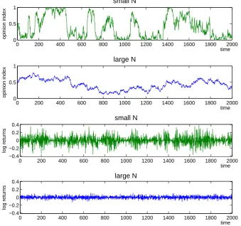
is known to be a convenient summary measure of the model properties with respect to an enlargement of system size. If the variance ofz remains con-stant (or even increases) when the system is enlarged, the leptokurtosis and volatility clustering of returns will be preserved in a standard Walrasian model of market clearing. A decreasing variance under enlargement of sys-tem size, on the other hand, is characteristic of self-averaging and thus leads to counter-factual Gaussian properties of returns, as shown in the bottom panel of Figure 1 and explained in more detail in the following section.
3
Financial Market Framework
0 200 400 600 800 1000 1200 1400 1600 1800 2000 0
0.5 1
time
opinion index
small N
0 200 400 600 800 1000 1200 1400 1600 1800 2000 0
0.5 1
time
opinion index
large N
0 200 400 600 800 1000 1200 1400 1600 1800 2000 −0.4
−0.2 0 0.2 0.4
time
log returns
small N
0 200 400 600 800 1000 1200 1400 1600 1800 2000 −0.4
−0.2 0 0.2 0.4
time
log returns
[image:9.595.120.460.133.451.2]large N
Figure 1: The two panels on the top illustrate the time evolution of aggregate opinion dynamics measured as the fraction of agents in one of the two states, say, z = n/N (top panel N = 500, a = 0.5, λ= 1, D =N; second panel
N = 10000, a = 0.5, λ = 1, D = 500). The two panels on the bottom exhibit the corresponding time series of returns generated from a Walrasian pricing function, as for instance in Eq. (13) of Section 3 (withκ= 1), where the level of excess demand depends onz. The bottom panel illustrates that an enlargement of system size under extensive transition rates will lead to counter-factual Gaussian returns and absence of volatility clustering.
1991, 1993; Alfarano et al., 2005; Alfarano and Lux, 2007; Alfarano et al., 2008; Alfi et al., 2009; Irle et al., 2011, for more realistic or detailed imple-mentations). Suppose that market participants are divided into two groups: the first group is populated by NF fundamentalists, who buy (sell) assets
when the price is below (above) its fundamental value PF. Their excess
des-ignates the sensitivity to deviations between the fundamental value and the market price P. Without loss of generality, the fundamental price is as-sumed to be constant over time. The second group is populated by NN T
noise traders, who are essentially driven by herd instincts in their investment strategies. Depending on their expectations of future price movements, noise traders can be eitheroptimists (subscript O)orpessimists (subscript P). The excess demand of the noise trader group will be proportional to their aggre-gated state, EDN T =γN T(NO−NP), whereNO and NP are the numbers
of optimists and pessimists, respectively, with NN T = NO+NP. The
pa-rameter γN T >0 governs the impact of the noise traders’ aggregate mood
on the asset price. In line with the notation of the previous section,EDN T
can be parameterized as a function ofz =NO/NN T, that is the fraction of
optimists over the total number of noise traders
EDN T =γN T ·NN T(2z−1). (9)
While the share of fundamentalists and noise traders is constant over time (so there are no transitions between those two groups), switches from optimism to pessimism and vice versa do take place among the noise traders, and are governed by the Markov chain detailed in Section 2. Hence noise traders change their opinions about the future prospects of an asset for idiosyncratic reasons or because of a tendency to follow the majority opinion of their peers. Assuming sluggish price adjustments by a market maker in the presence of excess demand, one typically formalizes the price dynamics as
dP
P ·dt =θ·ED=θ[EDF +EDN T], (10)
where θ is the speed of price adjustment. As an approximation to the re-sulting disequilibrium dynamics, one may consider instantaneous market clearing (θ→ ∞) or equivalently a Walrasian scenario (ED= 0) and solve (10) for the equilibrium price
P =PF exp
NN T ·γN T
NF ·γF
(2z−1)
=PFexp [κ(2z−1)], (11)
where
κ= NN T ·γN T
NF ·γF
Given a realization of the process z, we can see from (11) that periods of undervaluation (compared to the fundamental price) will alternate with episodes of overvaluation. In the first case the majority of noise traders are pessimists, while in the second case most are optimists.
Finally, returns are typically defined as the log-increment of prices
r(t,∆t) = log
P(t+ ∆t)
P(t)
=κ∆z , (13)
and the third panel of Figure 1 shows the corresponding time series of log-returns for a ‘small’ number of traders (NF =NN T = 500), visually already
indicating a leptokurtic return distribution and volatility clustering. In fact, Alfarano and Lux (2007) have shown that this very simple model quantita-tively reproduces the stylized facts of financial returns with (i) a fat-tailed distribution of returns, (ii) an absence of auto-correlation in raw returns, and (iii) a slowly decaying positive auto-correlation in even functions of re-turns, i.e.volatility clustering. Increasing the number of agents, for instance toNF =NN T = 10,000 (keeping D= 500) as shown in the bottom panel
of Figure 1, turns the abrupt mood swings inz into much smoother paths and results in counter-factual Gaussian fluctuations of returns.
4
Network Hierarchy and Core Weights
Essentially, we know that the relative communication range D/N in the transition rates (4) and (5) determines whether or not the model is self-averaging. Alfarano and Milakovi´c consider prototypical networks with bi-directional links, in particular regular lattices, random graphs, small-world networks of the Watts and Strogatz (1998) type, and the scale-free networks of Barab´asi and Albert (1999). Among these it is merely the random graph that exhibits a constant relative communication range since in that caseD=
N ℓ, whereℓdesignates the constant linking probability among agents in the random graph. On the other hand, D/N approaches zero for an increasing system size in the other network structures, unless one appropriately changes the respective parameters in the generating mechanisms of these networks.
Figure 2: A stylized representation of a hierarchical core-periphery network, where core agents (black; bi-directional links) influence each other in their opinion formation, while peripheral followers (grey; uni-directional links) simply mimic their respective core agents. This basically corresponds to a weighted version of Kirman’s original model.
random graph is not a convincing mapping of socio-economic relationships either, because it implies that the average connectivity of agents increases linearly with system size.3
Now suppose instead that N core agents are still bi-directionally linked among themselves, i.e. they still obey the Markov chain in Section 2. Additionally, each core agent has a constant number
W of followers in the periphery, with uni-directional links emanating from the core to the periphery. Uni-directional linking implies that the state of peripheral followers corresponds to the state of the respective core agents. Then the total number of followers isW N =F, with a total ofF+N agents in the entire network. In this case, the system-wide concentration of agents in stateX will be
z= W n+n
F+N =
n(W + 1)
N(W + 1) =
n
N, (14)
which just amounts to a relabeling of variables. Put differently, in this special case the system sizeF+N can be expanded at will by simply adding follow-ers F without encountering the self-averaging problem. Thus we preserve system-wide fluctuations in a population ofF+N individuals, although only
N socially interacting core agents are responsible for the fluctuations. At
3
A simple example illustrates this implausibility. Suppose you live in Smallville, where you closely interact with, say, thirty people. Moving to Metropolis, with a population about three hundred times the size of Smallville, a constant linking probability would imply that you now closely interact with a number of agents on the order of 105
the same time, the hierarchical structure avoids the empirically unsatisfac-tory random graph structure in the entire population that would otherwise be necessary to preserve non self-averaging fluctuations. The assumption of a constant number of followers per core agent, however, is quite arti-ficial and unsatisfactory. Therefore we want to investigate more general core-periphery structures by randomly drawing the number of followers per core agent from various distributions, keeping the total number of followers constant. We examine whether or how the dynamics of z change when the dispersion of followers increases. Notice that the respective numbers of fol-lowers now act as weights in the opinion formation process of core agents, otherwise we recover the unweighted and already well-understood cases re-sulting in the large-N limit of the generalized transition rates (4) and (5). Put differently, we would like to avoid the problem of self-averaging when enlarging the system, but without taking recourse to random graphs. There-fore we turn to core-periphery networks as a stylized representation of the institutional structure of financial markets, and investigate whether these hierarchical networks overcome the problem of self-averaging when the core remains small relative to the periphery.
5
Simulation Setup and Results
It is important to recall that we can study the (non) self-averaging property without actually increasing the number of agents in our subsequent simu-lations, because the addition of followers amounts to changing core agent
weights. Notice that adding core agents instead of followers would corre-spond to the scenario that Alfarano and Milakovi´c (2009) already studied in detail, where the structure of the bi-directional (core) network determines whether the model is self-averaging or not in the large N limit. The in-troduction of weights, however, prevents a straightforward application of their mean-field technique: when the weights are widely dispersed, the aver-age number of followers per core aver-agent obviously no longer provides a good approximation. Therefore we simulate the opinion dynamics in various core-periphery models, where we increase the dispersion of weights while drawing weights from different distributions, or altering the network structure in the core. We compare the resulting variance of z both to the mean-field pre-diction and to the variance in another limiting case that we have termed theindependent one-leader scenario below.4
After all, the variance ofzis a useful summary measure of the different scenarios because we know that if it decreases relative to the mean-field benchmark, the weighted core-periphery networks will still suffer from the problem of self-averaging. If on the other hand the variance ofz remains constant, the hierarchical model will be im-mune to self-averaging.
5.1 Network-adapted transition rates
To implement individual transition probabilities, in line with the transition rates (1) and (3), we first consider the (symmetric) adjacency matrixE =eij
for i, j ∈ {1, . . . , N} that keeps track of the links or edges between core agents, with eij = 1 if i and j are neighbors and eij = 0 otherwise.5 The
key element in the implementation of the transition rates is to determine for each agentithe number of neighbors that are in the opposite state, say ni.
Let e(i) denote the i-th column of the adjacency matrix E, which
ba-sically informs us of who is or is not an i-neighbor. While some of the neighbors will be in the same state as agenti, others will be in the opposite
4
Appendix A contains an analytical treatment of this case.
5
state, and these are the agents that we are interested in when implementing transition rates. To extract the i-neighbors that are in the opposite state, consider the projection matrix S(i) of dimension N ×N that keeps track of thei-neighbors that are in the opposite state: that is, for each ithe off-diagonal elements of S(i) are zero, sij = 0 if i 6= j, and obviously sii = 0
as well; on the diagonal ofS(i) we have sjj = 1 if the state of neighborj is
opposite to that of agenti, and sjj = 0 otherwise. Then the column vector k(i) =S(i) e(i) expresses which i-neighbors are in the opposite state, and
we finally haveni=kT(i)k(i).
Thusin the absence of followerswe would posit the transition probability ˜
πi = (a+λ ni)∆tfor switching states on the individual level. To ensure that
0 ≤ π˜i ≤ 1∀i, we need ∆t ≤ 1/(a+λ nmax), where nmax designates the
number of neighbors of the node(s) with the highest degree in the network. Since an agent can be connected at most to all other agents, we utilize the transition probability
˜
πi=
a+λni
a+λN (15)
for individual switches, hence agenti’s probability to remain in the current state is 0≤1−π˜i≤1.
In the presence of followers, we first need to make sure that our simula-tion results are comparable with the mean-field predicsimula-tion arising from (15), hence the individual transition probabilities need to be adapted to the core weights stemming from the hierarchical network setup. Let the column vec-torw, with elements wi, record the number of followers or weights for each
core agent i, soF =P
iwi is the total number of followers in the network,
and lethfi=F/N be the average number of followers per core agent. Now we are interested in the weighted sum of core agents who are in the opposite state of an agent i, denoted fi. Since k(i) describes the i-neighbors that
are in the opposite state, the weighted sum of core agents in the opposite state is straightforwardly computed as fi = kT(i) w = eT(i) S(i) w, and
the probabilitypi to observe a change in the state of agent iin the weighted
scenario is now given by
πi=
a+λfi/hfi
a+λN (16)
Notice several points about the formulation of the herding term in the nu-merator of (16). First, using the definition of hfi, we can rewrite it as
ensures 0≤πi ≤1∀i. Put differently, since 0≤ni ≤N, the weighted
for-mulation has the same boundaries as the unweighted one. Second, if all core agents have the same number of followers, we have that∀i fi=ni hfi, so we
recover the unweighted original formulation (15). Third, the ratiofi/hfiin
the sum of (16) is a direct measure of the dispersion of core weights, readily illustrating why we should not expect the mean-field approximation to be accurate when the dispersion becomes large.
5.2 Simulation setup
In our simulations, we fix the number of core agents atN = 500 and draw the number of followers from Gaussian, uniform, exponential and Pareto dis-tributions with meanhfi= 1000 such that each randomly drawn number is rounded to the nearest (absolute) integer value. LetN+
andF+
respectively denote the number of core agents and followers that are in the optimistic state. The system-wide concentration of agents in the optimistic state is now
z= (N+
+F+
)/M, whereM =N+F is the total number of agents. In all scenarios we set the parametersa, λ in such a way thatǫ= 1, which yields a uniform distribution ofzwithV ar(z) = 1/12≈.083 when the mean-field approximation applies. One ‘sweep’ of the system corresponds to one round of sequential updating of all core agents in the system, thus requiringN steps per sweep, and each simulation run consists of half a million sweeps. Finally, we successively increase the standard deviationσf of the respective
distribu-tion while ensuring that the weights remain positive and record the variance ofz for each sequence of increasing σf . Recall again that whenV ar(z)
in-creases (dein-creases) above (below) the “knife-edge” value of one twelfth, this implies that the distribution of z transforms from a uniform to a bimodal distribution with non-trivial averaging behavior (unimodal distribution with trivial self-averaging).
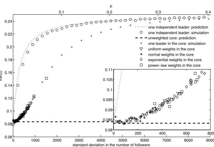
5.3 Core structure and one-leader benchmark
0 1000 2000 3000 4000 5000 6000 7000 8000 9000 0.06
0.08 0.1 0.12 0.14 0.16 0.18 0.2 0.22 0.24
standard deviation in the number of followers
Var(z)
one independent leader: prediction one independent leader: simulation unweighted core: prediction one leader in the core: simulation uniform weights in the core normal weights in the core exponential weights in the core power−law weights in the core
0 200 400 600 800
0.08 0.085 0.09 0.095 0.1 0.105 0.11
0.3
0.1 0.2 0.4
[image:17.595.126.469.125.361.2]p
Figure 3: The impact of increasing heterogeneity in core weights on system-wide volatility. The simulations (with a fully connected core D = N and behavioral parametersa=λ= 1, so ǫ= 1) demonstrate that rising hetero-geneity leads to increasing volatility, irrespective of the particular distribu-tion from which the weights are drawn.
dynamics of the system, thereby increasing the time during which the system is near one of the two extreme states. Hence hierarchical networks are not only immune to self-averaging, but actuallyamplify volatility in the system. It is noteworthy that the outcome does not depend on the functional form of the distribution from which the weights are drawn.
In order to determine the limit of the variance amplification, we consider an extreme case that we label as the one-leader scenario. In this case, we allocate an equal number of followers to all but one core agent (the leader), who is then assigned a weight such that the average number of followers corresponds again to hfi = 1000. Let 1/N < p < 1 denote the fraction of followers that are connected to the one-leader, such that the leader has pF
followers, and assume that the remaining (1−p)F followers are allocated with equal weight among theN−1 remaining core agents. Whenp= 1/N, all core agents have the same number of followers,F/N. Conversely when
new simulation run, we successively shift a larger number of followers to the leader by increasing p. The result is shown in Figure 3, with V ar(z) intuitively approaching a value of one-fourth since the leading agent will represent almost the entire system by itself, and cannot be influenced by others anymore. Thus its actions will consist of random switches between the two states, while the few remaining core agents mimic the leader’s behavior. Hence the system spends half its time in one state and half in the other, resulting in a variance of one-fourth.
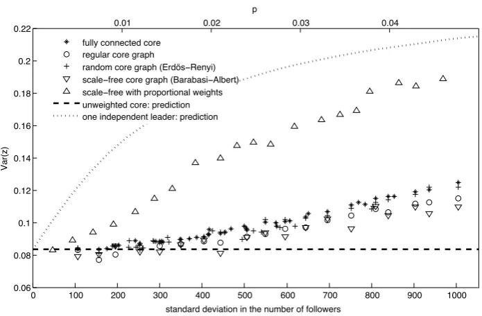
5.4 Varying the core structure
Our previous investigations show that a hierarchical network with a fully connected core not only overcomes the self-averaging problem, but also am-plifies volatility. A remaining issue is whether these results are robust with respect to the network structure in the core itself. On that account, we per-form another series of simulations with varying core network structures, and record how the different core networks respond to an increasing dispersion of weights.
0 100 200 300 400 500 600 700 800 900 1000 0.06
0.08 0.1 0.12 0.14 0.16 0.18 0.2 0.22
standard deviation in the number of followers
Var(z)
fully connected core regular core graph
random core graph (Erdös−Renyi) scale−free core graph (Barabasi−Albert) scale−free with proportional weights unweighted core: prediction one independent leader: prediction
0.01 0.02 0.03 0.04
p
Figure 4: The impact of different core network structures on system-wide volatility has merely second-order effects, except for the “proportional weights” scenario: if the core is a scale-free graph with core weights that are proportional to the degree of each agent in the core, the mean-field approx-imation immediately fails to produce accurate results and the variance ofz
rapidly increases, almost doubling compared to the other scenarios where core weights are still randomly assigned when varying the network structure in the core. As before, the simulations were conducted for N = 500 agents withλ= 1, andaand D set in such a way thatǫ= 1.
6
Conclusions
Hierarchical core-periphery structures turn out to overcome the problem of N-dependence in probabilistic herding models of the Kirman type. On one hand, this is good news from the viewpoint of the model’s asymptotic properties, because one is able to replicate the stylized facts of financial returns with behaviorally heterogeneous agents for any system size, without having to tune any of the behavioral parameters. On the other hand, our findings have somewhat stark implications from the viewpoint of investment strategy, and they also raise pressing new questions about the origins of hierarchical network structures.
[image:20.595.124.472.128.356.2]previously been considered as the exclusive source of volatility in social in-teraction models. If one accepts our premise that hierarchical networks are a useful representation of fund investor relationships in financial markets, then popular and traditional investment advice to ‘diversify one’s portfolio’ has to be judged with caution. Investors who are not wealthy enough to broadly diversify their portfolios, those who participate in funded retirement plans, or those who simply feel that they lack the skills or time to make appropriate investment decisions might very well delegate their investment decisions to institutional investors. But if these fund managers are socially interacting and influencing each other in their investment decisions, as the quoted em-pirical evidence suggests, this becomes a self-defeating strategy because we have argued that system-wide volatility increases under such circumstances. Put in more provocative terms, all the good intentions of investors to diver-sify risk can lead to the opposite effect if fund managers are prone to social interaction effects. Moreover, the presence of positive feedback effects in the time evolution of hierarchical networks seems to worsen the situation fur-ther, rather than improving it, since positive feedbacks would significantly increase the level of volatility in our simulations.
From the viewpoint of policy-making, our study indicates that a reduc-tion of financial volatility would be facilitated by a shrinking degree of hi-erarchical organization in financial markets, corresponding to an increasing decentralization of investment decisions. While such advice sounds straight-forward in principle, its implementation would most likely be more painful and complex: our results suggest that already very small values of p (or market share for that matter) lead to a sudden and pronounced increase in volatility. Keeping p very close to zero, on the other hand, would more or less imply getting rid of managed funds altogether, which hardly appears to be a feasible option.
References
S. Alfarano and T. Lux. A noise trader model as a generator of apparent financial power laws and long memory.Macroeconomic Dynamics, 11(S1): 80–101, 2007.
agent-based herding models.Journal of Economic Dynamics and Control, 33:78–92, 2009.
S. Alfarano, T. Lux, and F. Wagner. Estimation of agent-based models: The case of an asymmetric herding model. Computational Economics, 26: 19–49, 2005.
S. Alfarano, T. Lux, and F. Wagner. Time-variation of higher moments in a financial market with heterogeneous agents: An analytical approach.
Journal of Economic Dynamics and Control, 32:101–136, 2008.
V. Alfi, M. Cristelli, L. Pietronero, and A. Zaccaria. Minimal agent based model for financial markets i. European Physical Journal B, 67:385–397, 2009.
M. Aoki. Thermodynamic limits of macroeconomic or financial models: One- and two-parameter Poisson-Dirichlet models. Journal of Economic Dynamics and Control, 32:66–84, 2008.
A. V. Banerjee. A simple model of herd behavior. Quarterly Journal of Economics, 107(3):797–817, 1992.
A.-L. Barab´asi and R. Albert. Emergence of scaling in random networks.
Science, 286:509–512, 1999.
S. Bikhchandani, D. Hirshleifer, and I. Welch. A theory of fads, fashion, cus-tom, and cultural change as informational cascades. Journal of Political Economy, 100(5):992–1026, 1992.
S. Bornholdt. Expectation bubbles in a spin model of markets: Intermittency from frustation across scales. International Journal of Modern Physics C, 12:667–674, 2001.
W. A. Brock and C. H. Hommes. A rational route to randomness. Econo-metrica, 65:1059–1095, 1997.
C. P. Chamley. Rational Herds. Cambridge University Press, New York, 2004.
R. Cont. Empirical properties of asset returns: Stylized facts and statistical issues. Quantitative Finance, 1(2):223–236, 2001.
R. Cont and J. P. Bouchaud. Herd behaviour and aggregate fluctuations in financial markets. Macroeconomic Dynamics, 4:170–196, 2000.
E. Egenter, T. Lux, and D. Stauffer. Finite-size effects in Monte Carlo simulations of two stock market models. Physica A, 268:250–256, 1999.
X. Gabaix, P. Gopikrishnan, V. Plerou, and H. E. Stanley. A theory of power-law distributions in financial market fluctuations. Quarterly Jour-nal of Economics, 121(2):461–504, 2006.
U. Garibaldi, M. A. Penco, and P. Viarengo. An exact physical approach to market participation models. In R. Cowan and N. Jonard, editors,
Heterogeneous Agents, Interactions and Economic Performances, Lecture Notes in Economics and Mathematical Systems, pages 91–103. Springer, Berlin, 2003.
C. H. Hommes. Heterogeneous agent models in economics and finance. In L. Tesfatsion and K. L. Judd, editors, Handbook of Computational Eco-nomics, volume 2, pages 1109–1186. North-Holland, Amsterdam, 2006. H. Hong, J. D. Kubik, and J. C. Stein. Thy neighbor’s portfolio:
Word-of-mouth effects in the holdings and trades of money managers. Journal of Finance, 60:2801–2824, 2005.
G. Iori. A micro-simulation of traders’ activity in the stock market: the role of heterogeneity, agents’ interactions and trade friction. Journal of Economic Behavior and Organization, 49:269–285, 2002.
A. Irle, J. Kauschke, T. Lux, and M. Milakovi´c. Switching rates and the asymptotic behavior of herding models. Advances in Complex Systems, forthcoming, 2011.
A. Kirman. Epidemics of opinion and speculative bubbles in financial mar-kets. In M. P. Taylor, editor, Money and Financial Markets, pages 354– 368. Blackwell, Cambridge, 1991.
T. Lux and S. Schornstein. Genetic learning as an explanation of stylized facts of foreign exchange markets. Journal of Mathematical Economics, 41:169–196, 2005.
M. Newman. The structure and function of complex networks. SIAM Re-view, 45:167–256, 2003.
A. Pagan. The econometrics of financial markets. Journal of Empirical Finance, 3:15–102, 1996.
Y. Schwarzkopf and J. D. Farmer. Time evolution of the mutual fund size distribution. arXiv/0807.3800, 2008.
D. Stauffer and D. Sornette. Self-organized percolation model for stock market fluctuation. Physica A, 271:496–506, 1999.
D. J. Watts and S. H. Strogatz. Collective dynamics of ‘small-world’ net-works. Nature, 393:440–442, 1998.
R. Wermers. Mutual fund herding and the impact on stock prices. Journal of Finance, 54(2):581–622, 1999.
A
Independent One-Leader Benchmark
Let us start by considering an arbitrary agent in the fully connected core who is always in a fixed state and does not change opinion. As before, let 1/N < p < 1 denote the fraction of followers that are connected to the fixed-opinion agent, orindependent leader, such that the agent has pF
followers, and assume that the remaining (1−p)F followers are allocated with equal weight among the remaining core agents, indexed byi= 1, . . . , N−1. When p = 1/N, all core agents have the same number of followers, F/N. Conversely when p → 1, the system is almost entirely represented by the leader. For ease of notation, let us write the transition probability as
πi = (a+λN Fi/F) ∆t for i= 1, . . . , N −1, (17)
where Fi now denotes the system-wide number of followers in the opposite
indicator function that takes on the values 0 or 1 depending on whether the state of agent iequals or is different from the state of the fixed-opinion agent. Then we can rewrite the herding term in Eq. (17), N Fi/F, taking
into account the fixed opinion of the leader (say, being optimistic)
NFi F =
N F
F pβ+ (n−1)F(1−p)
N−1
, (18)
which yields the modified version of the transition probability (17),
πi =
a+λN pβ+λ N
N −1(1−p)n
∆t (19)
≈(a+λN pβ+λ(1−p)n) ∆t
for largeN. Depending on the value of the indicator function β, the transi-tion probabilities of agent iare either
πi = (ε+ (1−p)n)λ∆t or (20)
πi = (ε+N p+ (1−p)n)λ∆t , (21)
where we adapted ε to the definition (7) by noting that a fully connected core impliesD=N.
Fixing the opinion of one agent is equivalent to creating an asymmetry in the autonomous component that stems from the additional term N p in the modified transition rates. Put simply, the system exhibits a tendency towards the fixed opinion that depends on p. A straightforward mean-field argument (see, e.g., Alfarano and Milakovi´c, 2009) results in the following system-wide transition probabilities, analogous to an extensive version of the transition rates (4) and (5),
π− = n
N
ε+ (1−p)(N −n)
ε+N , (22)
π+
= (N −n)
N
ε+N p+ (1−p)n
ε+N . (23)
shorthands6
ε1=
ε+N p
1−p , ε2 = ε
1−p . (24)
Increasing the value of the control parameter p leads to an increasingly asymmetric distribution peaked around the opinion of the leader. Fixing the opinion of one agent, however, yields a very unsatisfactory approximation for the simulations in Section 5, where the leader is not in a fixed state but rather switches states as well. Therefore we proceed by assuming that the ‘independent’ leader switches opinion randomly, without being influenced by other agents, which basically means that the autonomous term in the mean-field transitions (22) and (23) is now stochastic and time-dependent, hinging on the random realizations of the leader’s state.
Such a situation is harder to tackle analytically because it leads to a stochastic differential equation with random coefficients. In order to ap-proximate the full mathematical problem, we employ a so-called adiabatic
approximation that neglects the adjustment of the system to the switch-ing of the leader by assumswitch-ing that the leader’s switches are slow enough in order for the N −1 agents to reach statistical equilibrium. Then we can consider the system as being in statistical equilibrium most of the time and, consequently, the resulting equilibrium distribution Ge becomes the
super-position of two independent equilibrium distributions, corresponding to the two possible configurations of the leader,
Ge=
1
2R(ε1, ε2;z) + 1
2R(ε2, ε1;z), (25) which is an average of the previous asymmetric distributions among the two alternative configurations of the leader. The equilibrium distribution is now symmetric (note the interchange of the parametersε1andε2) and U-shaped.
From Eq. (25), the second moment of the equilibrium distribution M2,e is
given by
M2,e =
1
2M2(ε1, ε2) + 1
2M2(ε2, ε1), (26) where M2(·,·) denotes the second moment of the respective asymmetric
Polya distribution with parameters ε1, ε2, and the variance of the
equilib-6
The Polya distribution converges to the Beta distribution for largeN. The results
rium distribution for a givenp is
V ar[z]p =
1
2V ar[ε1, ε2] + 1
2V ar[ε2, ε1] +1
2
M2
1[ε1, ε2] +M12[ε2, ε1] −
1 2
2
, (27)
where M1 designates the first moment of the respective asymmetric Polya
distribution, and 1/2 is obviously the mean of the equilibrium distribution
Ge. The two variances are equal since they are the same under an exchange
of the two parametersε1, ε2, hence the previous equation can be written as
V ar[z]p =V ar[ε1, ε2] +
1 2
M12[ε1, ε2] +M 2
1[ε2, ε1] −
1
4 . (28) It is possible to show (see, e.g., Garibaldi et al., 2003) that
M1[ε1, ε2] =
ε1
ε1+ε2
, (29)
V ar[ε1, ε2] =
ε1ε2
(ε1+ε2)2
ε1ε2+N
N(ε1ε2+ 1)
, (30)
and utilizing these in Eq. (28) yields
V ar[z] = 1 4 −
ε1ε2
(ε1+ε2)(ε1+ε2+ 1)
. (31)
Finally, recalling the shorthands in (24), we obtain the variance as a function of the control parameterp,
V ar[z]p =
1 4 −
1 +pN
(2 +pN)(3 +pN−p) , (32) under the parameter choice ε = 1, i.e. λ = 1 and a = 1. For N ≫ 1, we immediately see that Eq. (32) provides boundary values that are consistent with our previous findings: if p = 1/N, the variance tends to 1/12, repre-senting the correct value for the uniform distribution (recall the parameter choice ε= 1); if p → 1, the variance tends to 1/4, representing a distribu-tion concentrated either in 0 or 1. We simulated the modified model with a randomly switching leader, successively increasing the control parameter
sweeps.
The results, along with the prediction (32), are shown in Figure 3. For easier comparison with the simulation results in Figures 3 and 4, we calculate the standard deviation in the number of followers for each parametrization ofp, which is
σ=
s
1
N(pF)
2+N −1
N
(1−p)F N −1
2
−
F N
2
, (33)
and invert the relation to obtain
p= σ
√
N −1
F +
1
N. (34)