An Adaptive Response Compensation Technique for the Constant Current Hot Wire Anemometer

An Adaptive Response Compensation Technique for the

Constant-Current Hot-Wire Anemometer

Soe Minn Khine, Tomoya Houra, Masato Tagawa*

Department of Mechanical Engineering, Nagoya Institute of Technology, Nagoya, Japan Email: *_{[email protected]}

Received February 9, 2013; revised March 10, 2013; accepted March 18, 2013

Copyright © 2013 Soe Minn Khine et al. This is an open access article distributed under the Creative Commons Attribution License, which permits unrestricted use, distribution, and reproduction in any medium, provided the original work is properly cited.

ABSTRACT

An adaptive response compensation technique has been proposed to compensate for the response lag of the con- stant-current hot-wire anemometer (CCA) by taking advantage of digital signal processing technology. First, we have developed a simple response compensation scheme based on a precise theoretical expression for the frequency response of the CCA (Kaifuku et al. 2010, 2011), and verified its effectiveness experimentally for hot-wires of 5 μm, 10 μm and 20 μm in diameter. Then, another novel technique based on a two-sensor probe technique—originally developed for the response compensation of fine-wire thermocouples (Tagawa and Ohta 1997; Tagawa et al. 1998)—has been proposed for estimating thermal time-constants of hot-wires to realize the in-situ response compensation of the CCA. To demon- strate the usefulness of the CCA, we have applied the response compensation schemes to multipoint velocity measure- ment of a turbulent wake flow formed behind a circular cylinder by using a CCA probe consisting of 16 hot-wires, which were driven simultaneously by a very simple constant-current circuit. As a result, the proposed response com- pensation techniques for the CCA work quite successfully and are capable of improving the response speed of the CCA to obtain reliable measurements comparable to those by the commercially-available constant-temperature hot-wire anemometer (CTA).

Keywords: Flow Measurement; Hot-Wire Anemometer; Turbulent Flow; Constant-Current Hot-Wire Anemometer; Response Compensation; Frequency Response; Time-Constant; Multipoint Measurement;

Digital Signal Processing

1. Introduction

In recent years, particle image velocimetry (PIV) has become one of the most popular techniques for measur- ing velocity fields. The hot-wire anemometry [1-5], on the other hand, has long been used mainly for measuring turbulent gaseous flows because of its simple and highly- reliable measurement systems and wide range of appli- cability. Thus, the hot-wire anemometry is still frequen- tly utilized as a reliable research tool for statistical and frequency analyses of turbulent flows.

The hot-wire anemometry is generally driven at three operation modes, i.e., the constant temperature, constant- current and constant voltage modes. For the application of the hot-wire anemometry, the constant-temperature anemometer (CTA) is commercially available and almost always used as a standard system for driving the hot-wire, while the other two modes are rarely used, primarily due to their response lag during velocity fluctuation mea-

surement. However, the electric circuit of the CTA is not simple, and the measurement system is fairly expensive. On the other hand, the constant-current hot-wire ane- mometer (CCA) can be set up with a very simple and low-cost electric circuit for heating the hot-wire. Thus, if we improve the response characteristics of the CCA with the aid of digital signal processing, the CCA will have a great advantage over the CTA and will be a promising tool for multipoint turbulence measurement.

to-diameter ratio) is an important parameter characteriz- ing the response of the hot-wire. In our previous studies [6,7], we have successfully derived a precise theoretical solution for the frequency response of an actually-used hot-wire probe which consisted of a fine metal wire, stub parts (copper-plated ends/silver cladding of a Wollaston wire) and prongs (wire supports). As a result, we were able to find the geometrical conditions for the frequency response of the CCA to be approximated by the first- order lag system, which can be characterized by a single system parameter called the thermal time-constant [5].

If the time-constant value is known in advance, we may apply the existing response compensation tech- niques for the first-order system [4,5] to recover the re- sponse delay in the CCA measurement. In reality, how- ever, since the time-constant value of the CCA changes largely depending on flow velocity [8] and physical properties of the working fluid, it is very difficult to es- timate the time-constant value of the hot-wire accurately. In our previous papers [6,7], we proposed a digital re- sponse compensation scheme based on the precise theo- retical expression for the frequency response of the CCA. The results showed that the scheme worked successfully, reproducing high-frequency velocity fluctuations of a turbulent flow. However, this compensation scheme needs more information regarding the geometrical pa- rameters of the hot-wire probe, i.e., the diameters and lengths of the wire and stub together with their physical properties.

In the present study, first, we thoroughly tested the theoretical expression for the frequency response of the CCA by applying it extensively to the digital response compensation of three different hot-wire probes consist- ing of tungsten wires 5 μm, 10 μm and 20 μm in diameter. Secondly, we have proposed a novel approach to the re- sponse compensation of the CCA output that will work without our knowing in advance the geometrical pa- rameters of the hot-wire probe. This approach is based on a two-sensor probe technique for compensating the re- sponse delay of fine-wire thermocouples [9,10], and en- ables in-situ estimation of the time-constant values of the hot-wire probe, and will realize adaptive response com- pensation of the CCA outputs. Specifically, in the two- sensor probe technique, two hot-wires of unequal diame- ters—having different response speeds—are used simul- taneously, and the time-constant values of the two hot- wires can be obtained from the measurement data itself without carrying out any dynamic calibration of the hot- wire probe.

Finally, in order to demonstrate the usefulness of the CCA, we have applied the above response compensation schemes to multipoint velocity measurement of turbulent flows e.g., [11-13]. In the present multipoint measure- ment, we have simultaneously used 16 hot-wires driven

by the CCA to measure a turbulent wake flow formed behind a cylinder. In these verification experiments, we have measured turbulence intensities (r.m.s. values), power spectra and instantaneous signal traces of the ve- locity fluctuations, and have compared them with those obtained by a hot-wire probe driven by a commercially available constant-temperature hot-wire anemometer.

[image:2.595.317.531.573.718.2]

2. Time Constant of Hot-Wire for CCA

Mode

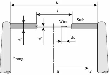
Figure 1 shows the geometrical features and coordinate system of the CCA probe used in the theoretical analysis (see Appendix A). As shown in Figure 1, the hot-wire is a fine tungsten wire (sensing part) with copper-plated ends (stubs) which are soldered to the prongs (wire sup- ports). By applying electric current I to the fine-wire element (length: dx, diameter d1), the generated Joule heat should balance with the sum of the following heat losses: heat convection, heat conduction, heat accumula- tion and thermal radiation. Since the heated wire is very fine, we can assume that the amount of heat radiation is negligible and the cross-sectional temperature distribu- tion is uniform [14]. Therefore, the energy balance equa- tion for the hot-wire can be written as (in this section, the subscript 1 for wire or 2 for stub is omitted for simpli- city):





2 2

a 2

π

,

T I R dh T

T T a

cS cS x

  



 _{   } 

  (1)

where  is time, R denotes the wire resistance per unit length and given by R  S [: electric resistivity,



_π 2 ₄



S  d : cross-sectional area of the wire], and I: electric current, h: heat transfer coefficient, T: wire tem- perature, Ta: ambient fluid temperature, a



 c



: thermal diffusivity of wire material, : thermal conduc- tivity, : density, c: specific heat. In Equation (1), R can be expressed as a linear function of the temperature difference between the wire and reference temperatures as:





a 1 a a

R_R_{ } T T_

 , (2)

where a is electric resistance per unit wire length at

the reference temperature and a denotes a temperature coefficient of wire material. Then, Equation (1) can be rewritten as:

R





2 2 2

a a a

a 2

π

.

I R dh I R

T

T T a

cS cS T x      _   _{   }    (3)

In hot-wire measurement, the effective cooling rate of the heated wire must principally be a function of flow velocity and can be obtained from the heat transfer coef- ficient of the fine wire, h, while the heat generation term is a nonlinear function of the electric current I and the wire resistance is determined by wire temperature as shown in Equation (2). To make Equation (3) theoreti- cally treatable, it needs to be linearized by decomposing the relevant physical quantities into a time-averaged component and a fluctuation one as: T T t h h h  ,   ,

I I i [1,15,16]. Then, we can obtain a governing equation of the constant-current hot-wire anemometer by formulating the energy balance equation with the fol-lowing procedures: 1) ignore the contribution of the se- cond- and higher-order fluctuation components; 2) derive a governing equation for the first-order fluctuation com-ponents by time-averaging the equation obtained in 1); 3) introduce a well-accepted correlation of to relate the heat transfer coefficient to the flow velocity; and 4) assume the electric current I to be constant. From the above procedures, the static and dynamic characteris-tics of the CCA are expressed as:

n

h A BU 





2 2 a a 2 1 0 d i

I R _{T T a} T

cS

d _,

x

 



    (4)





2 1

a 2

1 π n _,

i

t _{t a} t dBnU _{T T u} cS x           

  (5)

where _i is the thermal time-constant ( or 2), and is primarily related to the time-averaged heat transfer coefficient around the fine wire

1

i

h and electric current

I as follows:

2 a a

. π

cS dh I R

 

  

 (6)

In Equation (6), the heat transfer coefficient h can be expressed as a function of flow velocity U and is written as:

, n

h A BU (7) where the constants A, B and n can be obtained from the Collis-Williams correlation equation [17]; see Equation (A13). As seen from Equation (6), the time constant i should be a complex function of flow velocity U , driv- ing current I , wire diameter d, etc. Thus, in general, we

need to either obtain the time-constant value experimen- tally or estimate it empirically.

3. Response Compensation Techniques for

the CCA

3.1. Response Compensation Based on Precise Frequency Response Function

The frequency response of the hot-wire driven by the CCA, H1

 

 , has been derived theoretically by the

authors [6,7], and is expressed by the following equation

 













1,m 1 1 1

2,m 2 1,m 1 2,m 2 2

2 1 2

2

1 1

1 2

2 1 1 1

2 2 2 2

1

cosh

1 1 1 2

coth cosh

2 2 2

sinh 2

Z H

j

Z Z Z L

j j j

L L d d                       _  _  _                                          _{  }  _{  }      (8) To estimate theoretically the frequency response of hot-wires, we have applied Equation (8) to the three dif- ferent tungsten hot-wires (5 μm, 10 μm and 20 μm in diameter) with copper-plated ends (stubs). The geomet- rical parameters of the hot-wires are given in Table 1, in which ℓ/d1 and L denote the aspect ratio of the fine-wire and the distance between the prongs, respectively. All the hot wires have copper-plated ends 35 μm in diameter and are supported by the prongs (see Figure 1). In the present analysis, electric currents for the hot-wires driven at the CCA mode were set respectively at 40 mA, 100 mA and 260 mA for the 5 μm, 10 μm and 20 μm hot-wires, so as to provide adequate sensitivity to flow velocity. The air- flow velocity and fluid temperature were 7 m/s and 25˚C, respectively. Figure 2 shows the Bode diagram (gain) calculated from Equation (8). As shown in Figure 2, the frequency response of the hot-wire driven at the CCA mode can be naturally improved by decreasing the wire diameter. In the present calculation conditions, the 5 μm tungsten wire responded adequately to velocity fluctua- tions up to about 100 Hz without response compensation, while the response speed of the 20 μm wire decreased by an order of magnitude compared with the 5 μm one.

[image:4.595.56.287.121.346.2]

Table 1. Detailed features of three different hot-wires used. Definitions of the geometrical parameters d1, ℓ and L are

given in Figure 1.

d1 ℓ ℓ/d1 L

Material

[μm] [mm] [-] [mm]

Tungsten 5 1.5 300 5

Tungsten 10 2.0 200 6

Tungsten 20 4.0 200 7

Figure 2. Frequency response of CCA obtained from Equ- ation (8) as a function of length-to-diameter ratio (tungsten wires 5 μm, 10 μm and 20 μm in diameter). (see Appendix A).

cent of its length. In such a case, as seen from Figure 2, the frequency response of the hot-wire driven by the CCA can be approximated by the first-order lag system, whose response can be expressed as a function of only the time constant. If the aspect ratio becomes smaller than about 200, the cooling effects of the wire supports such as the stub and prong will emerge, and can deterio- rate the frequency response of the hot-wire. As a result, the Bode diagram for shorter wires behaves in a more complex manner (see Figure A1 in Appendix A).

The digital signal processing of the response compen- sation based on a known frequency-response function was described in detail in a previous paper [10]. The pro- cedure is applicable to the hot-wire measurement and can be summarized as follows: First, the hot-wire output (time-series data) is transformed into frequency-domain components using the fast Fourier transform (FFT). Next, each frequency component is multiplied by 1/H1 ()— the reciprocal of Equation (8)—to compensate for the output in the frequency domain. Finally, the inverse FFT is applied to the frequency-domain components thus cal- culated to obtain the compensated time-series data of the hot-wire output.

3.2. Response Compensation of CCA by Two-Sensor Technique

To use the above response compensation scheme based

on Equation (8), we need to know the geometrical parameters of the hot-wire probe. On the other hand, if the frequency response of the hot-wire can be repre- sented by the first-order lag system, we can apply the two-sensor technique, which does not need the geomet- rical parameters of the probe [9,10], to the response com- pensation of the CCA. In the present study, we used two methods called and . Their methods are given below. min

e Rmax

3.2.1. emin Method

The first-order lag systems of the two hot-wires driven by the CCA can be expressed as follows:

1 g1 1 1

2 g2 2 2

d _, d d

, d

U

U U

U

U U

  

 

  _

 

 



(9)

where Ui and Ug denote respectively raw output of the CCA (uncompensated velocity) and fluid velocity around the hot-wire, and  and i are the time and time-constant defined by Equation (6), respectively. The subscripts

1

i and 2 denote two unequal hot-wires different in diameter. Ideally, the fluid velocities surrounding the two hot-wires, Ug1 and Ug2, must be expressed as





U U U

U U

g1 g2 g . In reality, however, the finite spatial resolution between the two hot-wires and the instrumen- tation noise may change the relation between Ug1 and Ug2 as _g1 _g2. Thus, the time constants 1 and 2 can be determined so as to minimize the mean square value of the difference between Ug1 and Ug2, which is given by





2

g2 g1 .

e U U (10) The time-constant estimation method thus obtained was originally proposed by Tagawa and Ohta [9]. In what follows, we call this estimation scheme the “emin method”. Then, the time constants 1 and 2 can be ob- tained from the simultaneous equation derived from Equation (10) by minimizing the value of e. The result is given by the following equations:









2

2 1 21 1 2 2 21

1 _{2 2} 2

1 2 1 2

2

1 2 1 21 1 2 21

2 _{2 2} 2

1 2 1 2

,

,

G G U G G G U

G G G G

G G G U G G U

G G G G







    

 



  _



     

 _

  _

(11)

where G is the time derivative of U G



dU td



and 21 2– 1

U U U

  .

3.2.2. Rmax Method

[image:4.595.352.525.582.657.2]

measurement system, we can take another approach to estimate the time-constant values by maximizing the correlation coefficient R between Ug1 and Ug2:

g1 g2 2 2 g1 g2 , U U R U U   

  (12)

where the prime denotes a fluctuating component. By solving a simultaneous equation thus derived, we obtain the time constants 1 and 2 as a solution of quadratic equations:









2

1 1 1 1

2

2 2 2 2

4 2,

4 2.

B B C

B B C

       _        (13)

The quantities and C2 in Equation (13) are given by 1 2 1

, ,

B B C



 





 



1 2 2 1 1 2 2 1 1

1 2 2 1

1 2 2 1 1 2 2 1 2

1 2 2 1

1 2 2 1 1

1 2 2 1

1 2 2 1 2

1 2 2 1

,

,

,

,

a d a d b c b c B

b d b d a d a d c b c b B

c d c d a c a c C

b d b d a b a b C

c d c d

    _  _           _  _      _  _  (14)

and all the elements in Equation (14) are given by

2

1 1 1 2 1 2 1 1

2

2 2 2 1 1 2 2 2

2

1 1 1 1 2 1 2 1

2

2 2 1 2 1 2 2 2

2

1 1 1 2 1 1 2 1

2

2 2 1 2 2 1 2 2

1 1 1 1 2 2 1 1

, , , , , ,

a U G U U U G U

a U G U U U G U

b G U G U U U G

b U G G G U G U

c U G G G U G U

c G U G U U U G

d G U G G G U G

                                                                       

    2

2

2 2 2 1 2 1 2 2

, .

d G U G G G U G

                         _ (15)

In the present study, we have mainly used this ap- proach called the “Rmax method” [10]. It is noted that the time derivatives in Equations (11) and (15) can be ob- tained from the coefficients of a polynomial curve-fitting [18] for the digitized outputs of the two unequal hot- wires driven at the CCA mode.

4. Experimental Apparatus and

Measurement System

4.1. Single-Sensor and Two-Sensor Probes

In this experiment, we used three fine tungsten wires 5

μm, 10 μm and 20 μm in diameter for the CCA, and a 5 μm tungsten wire for the CTA, which was used as a ref- erence sensor. The detailed features of the fine-wires are given in Table 1. For the two-sensor technique, we have constructed two types of the CCA probes—one is the combination of 5 and 10 μm hot-wires, and the other is that of 10 and 20 μm ones. The schematic diagram of the constant-current circuit for driving a 5 μm or 10 μm wire is shown in Figure 3(a), and that for a 20 μm wire in

Figure 3(b). The driving circuit for 5 μm and 10 μm wires is very simple and can be composed at quite a low cost. On the other hand, a different circuit (shown in

Figure 3(b)) should be used for a 20 μm wire, since the current needs to be kept accurately constant even in case of a higher electric current. The later circuit, of course, can be used for driving a thinner wire, and is still much simpler to operate than the constant-temperature ane- mometer. The configuration and arrangement of the hot- wires consisting of single-sensor and two-sensor probes are shown (circled) in Figure 4. We have determined a proper wire separation so as to minimize thermal and

15 V

5 or 10 m

CCA Output

+

R

Rw

-R >> -Rw

(a) 2SC4736-AY 3 2 1 LF356N 1.5V 5 V + -Rw

20 m

[image:5.595.345.495.350.623.2]

CCA R Output 15 V LF356N 2SC4736-AY (b)

[image:5.595.112.234.440.585.2]

2

6

7 4 Stub

(copper, 40 m)

1.5

5

80

80

0.6

x y z

0

50 Flow

10 mm

Hot-wire probe CCA driving circuit

or CTA unit

Amplifier

circuit A/D converter

To Personal computer

CTA or CCA

(Tungsten, 5 m)

Hot-wire1

(Tungsten, 10 m)

Hot-wire2

(Tungsten, 20 m)

Prong (soldered)

y z

Single-sensor probe Two-sensor probe

2

6

7 4 Stub

(copper, 40 m)

1.5

5

80

80

0.6

x y z

0

50 Flow

10 mm

Hot-wire probe CCA driving circuit

or CTA unit

Amplifier

circuit A/D converter

To Personal computer

CTA or CCA

(Tungsten, 5 m)

Hot-wire1

(Tungsten, 10 m)

Hot-wire2

(Tungsten, 20 m)

Prong (soldered)

y z

[image:6.595.148.448.83.283.2]

Single-sensor probe Two-sensor probe

Figure 4. Experimental apparatus and details of hot-wire probes (single-sensor and two-sensor probes). The 10 μm and 20 μm hot-wire sensors shown in the two-sensor probe can be used for the single-sensor probe. For the two-sensor probe, we employed two combinations: Probe 1 is the combination of 5 μm and 10 μm hot-wires; Probe 2 (circled) is that of 10 μm and 20 μm ones. (All dimensions in millimeters.)

fluid-dynamical interferences between the two hot-wires.

4.2. Experimental Apparatus and Measurement System

As shown in Figure 4, the flow field to be measured is a turbulent far wake of a circular cylinder, and the test section is the mm region in the central plane

at 0 y



z0 mm



x D8. A uniform airflow up to 12 m/s can be produced using an upright wind tunnel with a two-dimensional contraction (contraction ratio, 5:1), and approaches to the cylinder set at the wind tunnel exit. It is noted that 5% - 10% free stream turbulence is generated by a perforated plate (hole size:  5 mm; staggered arrangement with 7 mm pitch). In the present experiment, the uniform airflow velocity was set to 7 m/s.

All the outputs of the hot-wires driven by the constant- current circuits shown in Figure 3 are amplified by 100 - 500 times and digitized by a 14-bit A/D converter (Mi- croscience ADM-670 and/or 681PCI). The sampling frequency is set at 10 kHz and the number of samples is 132,000 for each measurement. A personal computer (EPSON Endeavor Pro3100) is used to store the hot-wire outputs of the A/D converter and perform all the data processing. The hot-wire outputs are calibrated with the aid of a pitot tube in the range of 1 to 10 m/s.

5. Results and Discussion

5.1. Theoretical Response Compensation for Single-Sensor Measurement

First, we estimated the frequency response of the hot-

wires 5 μm, 10 μm and 20 μm in diameter to apply the theoretical response compensation scheme mentioned in section 3.1 to the CCA outputs.

Naturally, the mean velocity profiles obtained by these three hot-wires show little difference (a sample velocity profile is seen in Figure 5). Then, we appraised experi- mentally the effectiveness of the theoretical response compensation of the CCA on the basis of the turbulence intensities (root-mean-square values) and power spectra of the velocity fluctuations of the turbulent wake flow. The results are shown in Figures 6 and 7. Figure 6

Figure 5. Mean velocity profiles of single-sensor measure- ment by CTA and multipoint measurement by CCA (see Section 6.2). Cylinder is positioned at y = 0 mm.

Figure 6. Comparison of rms velocity profile between sin- gle-wire CCA measurements by 5 μm, 10 μm and 20 μm hot-wires and reference measurement by CTA.

[m

−

2·s

−

1]

Figure 7. Power spectra of velocity fluctuations measured using three single-sensor probes driven by CCA and that by CTA at y = 16 mm where the turbulent intensities take their maxima.

μm hot-wire outputs, respectively. As seen from the above, the proposed theoretical response compensation scheme works quite well.

5.2. Adaptive Response Compensation by the Two-Sensor Technique

Before applying the two-sensor technique to the present

experiment, we investigated the frequency response of the three hot-wires 5 μm, 10 μm and 20 μm in diameter to confirm that the response characteristics of these hot- wires can be approximated by the first-order lag system as explained in Section 3.1. Then, we estimated the time- constant values by the emin and Rmax methods described in Section 3.2. The results obtained at y = 16 mm are sum- marized in Table 2. As seen from Table 2, the time- constant values estimated by both Probe 1 and Probe 2 using the Rmax method are in good agreement with those obtained from the correlation equation proposed by Collis and Williams [17]. Figure 8 shows the compen- sated r.m.s. velocity distributions obtained by Probe 2 using the Rmax method (results obtained by Probe 1 is omitted due to space limitation). As seen from Figure 8, the present response compensation scheme works suc- cessfully and can provide acceptable results that are comparable to the CTA measurements, except the cen- terline region around y = 0 mm. This slight discrepancy near the centerline may be caused by an increase of thermal and/or fluid-dynamic interferences between the two hot-wires of the two-sensor probe shown in Figure 4.

The power spectra of both uncompensated and com- pensated velocity fluctuations measured at y = 16 mm are shown in Figure 9, where we also compared their dis- tributions with those obtained by the CTA. In the present Table 2. Time-constant values estimated from eminmethod, Rmax method and Collis-Williams law given by Equation

(A13) (y = 16 mm).

Probe 1



U5.0 m/s



Probe 2



U5.5 m/s



Scheme _

1 [ms]

d1: 5 μm

2 [ms]

d2: 10 μm

1 [ms]

d1: 10 μm

2 [ms]

d2: 20 μm

emin method 0.57 2.07 1.64 6.20

Rmax method 0.66 2.13 2.06 7.55

From Equation

(A13) 0.64 2.12 2.02 7.47

[m

−

2·s

−

1]

Figure 9. Comparison of power spectrum distribution using two-sensor technique using Rmax method (Probe 2).

experiment, we removed high-frequency noise compo- nents in the compensated CCA outputs using a finite-im- pulse-response (FIR) digital filter with the cutoff fre- quency of 3 kHz for the 10 μm hot-wire and 2 kHz for the 20 μm one. As seen from Figure 9, the power spectra of the compensated CCA outputs agree well with the CTA result, and high-frequency velocity fluctuations up to around 2 kHz can be well reproduced. Meanwhile,

Figure 10 shows a comparison of the instantaneous sig- nal trace between the uncompensated and compensated CCA outputs measured at y = 16 mm, with a reference of the CTA output. The CTA and CCA outputs were mea- sured independently (they are not simultaneous mea- surements). As seen from Figure 10(b), high-frequency velocity fluctuations have been recovered properly by the present response compensation scheme. As a result, the compensated CCA signal traces are analogous to the CTA one shown in Figure 10(a).

6. Application of Response Compensation

Technique to Multi-Sensor Measurement

6.1. Multi-Sensor Probe

Multipoint measurement and analysis will help us elu- cidate the spatiotemporal structures of turbulent flows. Thus, in the present study, we have explored the possi- bilities of applying the above-mentioned response com- pensation scheme to the multi-sensor probe driven at the CCA mode, since the constant electric-current circuit driving the hot-wires, e.g., Figure 3(a), is much simpler and can be constructed at an even lower cost than the constant-temperature anemometer (CTA). Figure 11

shows the photographs of the multi-sensor probe con- structed in our laboratory. As shown in Figure 11, six- teen tungsten hot-wires 5 μm in diameter with copper plated ends are aligned at intervals of 2 mm and soldered on steel prong tips. The configuration of the 5 μm hot- wire is the same as that given in Table 1, and the entire length of the sensing part becomes 30 mm. The present

(a)

(b)

Figure 10. Instantaneous signal traces of velocity fluctua- tions: (a) CTA measurement by single-sensor probe; (b) CCA measurements by two-sensor probe. The CTA and CCA outputs were measured independently (they are not simultaneous measurements).

muti-sensor probe was designed so as to measure ade- quately the turbulent far wake of a cylinder (Figure 4). The probe was set at the same height as the above ex- periment with the probe tip positioned at

y = 0 mm. When the airflow velocity at the wind-tunnel exit is 7 m/s and the probe is set at



x80 mm



8

x D (cylinder diameter: D = 10 mm), the mean velocity profile in the

y-direction can be sufficiently covered by the measure- ment range of 0  y  30 mm. We used the con- stant-current circuit shown in Figure 3(a) for driving the sixteen tungsten hot-wires 5 μm in diameter.

6.2. Multipoint Measurement

The multipoint measurement by the 16-channel CCA probe was performed in the turbulent far wake of the cylinder (Figure 4). Figure 5 shows the comparison be-tween the mean velocity profile measured by the multi-sensor probe and that obtained using the single hot-wire driven by the CTA. As seen from Figure 5, the uncompensated (raw) mean velocities of the multipoint measurement are almost coincident with the CTA meas- urements. Naturally, as for the measurement of the mean velocity profile, the response compensation scheme need not necessarily be applied to the CCA outputs. Mean- while, Figure 12 shows the comparison of r.m.s. velocity distributions between the multipoint measurements and the CTA result. In the present response compensation, the frequency components higher than 4.5 kHz were at- tenuated by a finite-impulse-response (FIR) digital low- pass filter. As seen from Figure 12, the r.m.s. velocities of the multisensor measurements compensated by using Equation (8) are in good agreement with those obtained by the CTA. Thus, a multi-sensor probe with the present response compensation scheme (Section 3.1) will work successfully to detect spatiotemporal behaviors of turbu- lent flow fields.

The instantaneous signal traces measured by the multi- sensor probe are shown in Figure 13. Figure 13(a)

shows the uncompensated (raw) outputs of the 16 hot-

Figure 12. Comparison of Rms velocity distributions of sin- gle-sensor measurement by CTA and multipoint measure- ment by CCA.

(a)

(b)

Figure 13. Instantaneous signal traces of multipoint meas- urement: (a) Uncompensated (raw) outputs; (b) Compen- sated results by theoretical response compensation scheme using Equation (8).

wires of the multi-sensor probe, in which the hot-wires are arranged at the constant intervals of 2 mm, and the cylinder was placed at y = 0 mm (see Figures 11 and 12). As seen from Figure 13(a), the mean velocity changes largely in the region of 0  y  20 mm, and the mean velocity gradient in the y direction is barely observed in the region of y  20 mm. On the other hand, Figure 13(b) shows the compensated signal traces. As seen from

Figure 13(b), the response compensation has reproduced high-frequency velocity fluctuations and has made it evi- dent that large-scale fluid motions exist through the shear layer of the turbulent far wake of the cylinder. Thus, the multi-sensor probe driven by the CCA together with the digital response compensation scheme will provide a useful tool for investigating spatiotemporal structures of turbulent flows.

7. Conclusion

response compensation scheme based on the frequency response function of the CCA [6,7], and verified its ef-fectiveness experimentally. Furthermore, another novel technique based on the two-sensor probe technique has been proposed, which enables in-situ estimation of the thermal time-constants of the hot-wires driven at the CCA mode to realize reliable response compensation of the CCA. To demonstrate the usefulness of the CCA, we applied the response compensation schemes to multipoint velocity measurement of the turbulent far wake of the circular cylinder by using the multi-sensor probe con- sisting of 16 hot-wires driven simultaneously by the very simple constant-current circuit. As a result, the proposed response compensation techniques for the CCA worked quite successfully and are capable of improving the re- sponse speed of the CCA to obtain reliable measure- ments comparable to those by the commercially-avail- able constant-temperature hot-wire anemometer.

8. Acknowledgements

ank Dr. K. Kaifuku for his

REFERENCES

[1] J. O. Hinze, ion, McGraw-Hill,

Hot-Wire Anemometry,” Annual Re-The authors would like to th

valuable assistance and advice with the theoretical re- sponse compensation scheme. This work was partially supported by a Grant-in-Aid for Scientific Research (No. 22560194) and for Young Scientists (No. 24760164) from The Japan Society for the Promotion of Science (JSPS).

“Turbulence,” 2nd Edit New York, 1975.

[2] G. Comte-Bellot, “

view of Fluid Mechanics, Vol. 8, 1976, pp. 209-231.

doi:10.1146/annurev.fl.08.010176.001233

[3] G. Comte-Bellot, “Springer Handbook of Experimental

y, “Hot-wire Anemometry,” Oxford University

Anemometry - Principles and

fuku, S. M. Khine, T. Houra and M. Tagawa,

e, T. Houra and M. Tagawa,

“Re-ment of the Transfer Function Hot-Fluid Mechanics,” In: C. Tropea, A. L. Yarin and J. F. Foss, Eds., Sec 5.2.1-5.2.7, Springer, Berlin, 2007, pp. 229-283.

[4] A. E. Perr

Press, New York, 1982. [5] H. H. Bruun, “Hot-Wire

Signal Analysis,” Oxford University Press, New York, 1995.

[6] K. Kai

sponse Compensation of Constant-Current Hot-Wire Ane- mometer,” Proceedings of the 21st International Sympo- sium on Transport Phenomena, Kaohsiung, 2-5 Novem- ber 2010, pp. 816-822.

[7] K. Kaifuku, S. M. Khin

sponse Compensation for Constant-Current Hot-Wire Anemometry Based on Frequency Response Analysis,” Proceedings of ASME/JSME 2011, 8th Thermal Engi- neering Joint Conference, Honolulu, 13-17 March 2011, Article ID: T10164.

[8] I. Kidron, “Measure

Wire and Hot-Film Turbulence Transducers,” IEEE Tran- sactions on Instrumentation and Measurement, Vol. 15, No. 3, 1966, pp. 76-81.doi:10.1109/TIM.1966.4313512 [9] M. Tagawa and Y. Ohta, “Two-Thermocouple Probe for

Fluctuating Temperature Measurement in Combustion— Rational Estimation of Mean and Fluctuating Time Con- stants,” Combustion and Flame, Vol. 109, No. 4, 1997, pp. 549-560.doi:10.1016/S0010-2180(97)00044-8 [10] M. Tagawa, T. Shimoji and Y. Ohta, “A Two-Thermo-

couple Technique for Estimating Thermocouple Time Con- stants in Flows with Combustion: In Situ Parameter Iden- tification of a First-Order Lag System,” Review of Scien- tific Instruments, Vol. 69, No. 9, 1998, pp. 3370-3378.

doi:10.1063/1.1149103

[11] R. F. Blackwelder and R. E. Kaplan, “On the Wall Stru- cture of the Turbulent Boundary Layer,” Journal of Fluid Mechanics, Vol. 76, No. 1, 1976, pp. 89-112.

doi:10.1017/S0022112076003145

[12] M. N. Glauser and W. K. George, “Application of Multi- point Measurements for Flow Characterization,” Experi- mental Thermal and Fluid Science, Vol. 5, No. 5, 1992, pp. 617-632.doi:10.1016/0894-1777(92)90018-Z

[13] T. Houra and Y. Nagano, “Spatio-Temporal Turbulent Structures of Thermal Boundary Layer Subjected to Non- Equilibrium Adverse Pressure Gradient,” International Journal of Heat and Fluid Flow, Vol. 29, No. 3, 2008, pp. 591-601.doi:10.1016/j.ijheatfluidflow.2008.03.004 [14] K. Kato, K. Kaifuku and M. Tagawa, “Fluctuating Tem-

perature Measurement by a Fine-Wire Thermocouple Pro- be: Influences of Physical Properties and Insulation Coa- ting on the Frequency Response,” Measurement Science and Technology, Vol. 18, No. 3, 2007, pp. 779-789.

doi:10.1088/0957-0233/18/3/030

[15] J. D. Li, “Dynamic Response of Constant Temperature Hot-Wire System in Turbulence Velocity Measurements,” Measurement Science and Technology, Vol. 15, No. 9, 2004, pp. 1835-1847.doi:10.1088/0957-0233/15/9/022 [16] A. Berson, G. Poignand and P. Blanc-Benon and G.

Comte-Bellot, “Capture of Instantaneous Temperature in Oscillating Flows: Use of Constant-Voltage Anemometry to Correct the Thermal Lag of Cold Wires Operated by Constant-Current Anemometry,” Review of Scientific In-struments, Vol. 81, No. 1, 2010, Article ID: 015102.

doi:10.1063/1.3274155

[17] D. C. Collis and M. J. Williams, “Two-Dimensional Con- vection from Heated Wires at Low Reynolds Numbers,” Journal of Fluid Mechanics, Vol. 6, No. 3, 1959, pp. 357- 384.doi:10.1017/S0022112059000696

[18] M. Tagawa, S. Nagaya and Y. Ohta, “Simultaneous Mea- surement of Velocity and Temperature in High-Tem- perature Turbulent Flows: A Combination of LDV and Three-Wire Temperature Probe,” Experiments in Fluids, Vol. 30, No. 2, 2001, pp. 143-152.

doi:10.1007/s003480000149

ta, “Response Compensa-[20] M. Tagawa, K. Kato and Y. Oh

tion of Fine-Wire Temperature Sensor,” Review of Scien-tific Instruments, Vol. 76, No. 9, 2005, Article ID: 094904. [21] M. Tagawa, K. Kato and Y. Ohta, “Response Compensa-

tion of Thermistors: Frequency Response and Identifica- tion of Thermal Time Constant,” Review of Scientific In-struments, Vol. 74, No. 3, 2003, pp. 1350-1358.

Appendix A: Theoretically-Derived

Frequency Response Function of the CCA

In this appendix, we have summarized the theoretical derivation processes of the frequency response function of the hot-wire probe, consisting of a fine metal wire, stub parts (copper-plated ends/silver cladding of a Wolla- ston wire) and prongs (wire supports) (see Figure 1).

Equation (5) should be a fundamental equation for obtaining the frequency response function expressed by Equation (8). In the right-hand side of Equation (5), the term



T T1– a



representing the time-averaged tempera- ture difference between the wire and surrounding fluid varies as a function of x. In the present analysis, however, we assume this term to be constant for simplicity and replace T1 by the spatially-averaged temperature along the wire T1,m, and similarly T2 by T2,mfor the stub. As

a result, the responses of the wire and stub temperatures to the velocity fluctuation u and the relevant boundary conditions are written as:

 Wire



0 x 2



:



2 1

1 1 1 1

1 1 2 1,m a

1 1 1 1

π

1 n _.

t _{t a} t d B nU _{T T u} c S x           

 



(A1)

 Stub



2 x L 2



:



2 1

2 2 2 2

2 2 2 2,m a

2 2 2 2

π

1 n _.

t _{t a} t d B nU _{T T u}

c S x

  



 _{  }  _{ }

 



(A2)

 Boundary conditions for Equations (A1) and (A2):

1

1 2

2 1 2 2

1 1 2 2

2 i) 0 : 0,

ii) 2 : ,

π π

iii) 2 : ,

4 4

iv) 2 : 0.

t x

x

x t t

t t

x d d

x x

x L t

      _  _      _{ }         _   (A3)

The boundary conditions 1) - 4) shown in Equation (A3) are formulated so as to represent the following physical requirements: 1) a temperature distribution along the heated wire is symmetrical about the origin of the x

axis



x0



; 2) at the interface



x2



, the tem- perature of the wire is equal to that of the stub; 3) heat flowing through the interface



x 2



is assumed to be conserved; and 4) the temperature at the tip of the prong (namely, temperature of the stub at x L 2) is kept at fluid temperature Ta.

In the following, we investigate theoretically the fre- quency response of the CCA along the lines of the pro- cedure used in the analyses of the frequency response of a fine-wire temperature sensor [19,20] a thermistor [21]. The temperatures of the wire and the stub, and

, and the flow velocity 1



,

t  x

 





 





 

 

1 1 2 2 ˆ

, e , d

ˆ

, e , d

ˆ

e d ,

j t

j t

j t

t x t x

t x t x

u u    , ,                         







(A4)

where j is an imaginary unit and an angular frequency



2πf



. From Eq. (A4), Equations (A1) and (A2) are transformed into the following equations:





_

_

_{ }









 

1 1 1,m

1

1 1

2 2 2,m

2

2 2

ˆ , ₁

ˆ , ˆ ,

ˆ _{, 1}

ˆ , ˆ ,

t x jω Z

t x u

a a

t x jω Z

t x u

a a  _      _        _{  }         _{    }  _  _ (A5)

where Z_i,m



i1, 2



is represented by



1

,m ,m a

π

. n

i i

i i

i i i

d B nU

_

Z T T

c S

 

  (A6)

Equation (A5) is composed of the two differential equations on the variable (coordinate) x, and their solu- tions are given by





 





 

1 1

2 2

1,m

1 1 2 2

1 1

2,m

2 3 4 2

2 2

ˆ , e e ˆ ,

ˆ , e e ˆ

x x

x x

Z

t x C C u

a Z

t x C C u

a               ,           _  _ (A7)

where C1C4 are the undetermined coefficients, and



1, 2



i i

  is defined by

2 2 2 2

1

1 _{1 1 1}

2 i i i i i i i i j a j a              _     _

 1 .

(A8)

The boundary conditions 1) - 4) in Equation (A3) are also written in the Fourier integrals, and are used to de- termine the coefficients C₁C₄ in Equation (A7). As a result, the frequency component of the wire temperature,

, becomes 1

ˆ

t









1,m

 

1 1 2

1 1

ˆ , 2 cosh Z ˆ

t x k x u

a ,

 _   _ 



  (A9)

where k is given by













2,m 1,m 2,m 2

2 2 2

2 2 1 1 2 2

2 1

1 2

2

1 1 1 1

2 2 2 2

cosh 2

2 cosh cosh

2 2

2 sinh sinh

2 2

Z Z Z L

k

a a a

L L d d          _ _ _                                      _              (A10)







2 ,

t  x u

 

 can be written

It is assumed that the wire temperature T1 can be re- placed by the mean temperature T1,m spatially-averaged

in the range of 2 x 2



. Therefore, we may ap- praise the frequency response of the wire by averaging

in the same range and the result



1

ˆ ,

t  x tˆ1,m

 

 is

described as follow:

 





 

/ 2 1,m _{/ 2}1

1,m 1

2

1 _{1 1}

1

ˆ ˆ , d

2 _{sinh ˆ}

2 2

t t x x

Z

k _u

a

 

 





  

_ _ __ 





 



 

    

(A11)

From the above Equation (A11), we finally obtain the frequency response of the hot-wire probe driven by the CCA, H1

 

 tˆ1,m

   

 uˆ  . The result is given by Equation (8). Similarly, the frequency response of the stub H₂

 

 _tˆ_2,m

   

 uˆ  _ can be obtained by de- termining the values of and in Equation (A7)

(not shown). 3

C C₄

If there is no stub (i.e., L), the wire is directly connected to the prong. Equation (8) is reduced to the following simple expression:

 

1

1,m

1 2

1 1 1

tanh 2 1

2 Z

H

a



  

 

 _{ }



  



  

 

 



 .



 (A12)

To investigate the frequency response of the CCA us- ing Equation (8), we need to evaluate the heat transfer coefficient h that plays a key role in determining the time constants 1 and 2 as shown in Equation (6). In the pre- sent study, we use the well-known Collis-Williams cor- relation equation [17], which is given by





0.17

0.45 f

a

Nu 0.24 0.56 R

0.02 Re 44 T

T



 

 

 

 

 

e ,

(A13)

where Nu and Re are the Nusselt and Reynolds numbers, respectively and are defined as Nuhd a and

a

ReUd  (U: flow velocity; a: kinematic viscosity of fluid); and Tf is a film temperature defined as





f a 2

T  T T (T: surface temperature of the wire). In the following, we investigate in detail the frequency re- sponse characteristics of the CCA to obtain basic know- ledge of the response compensation of its output. As for the hot-wire probe to be analyzed, a fine tungsten wire 5

m in diameter is supported by copper stubs 35 m in diameter, and the end of the stub is connected to the prong tip.

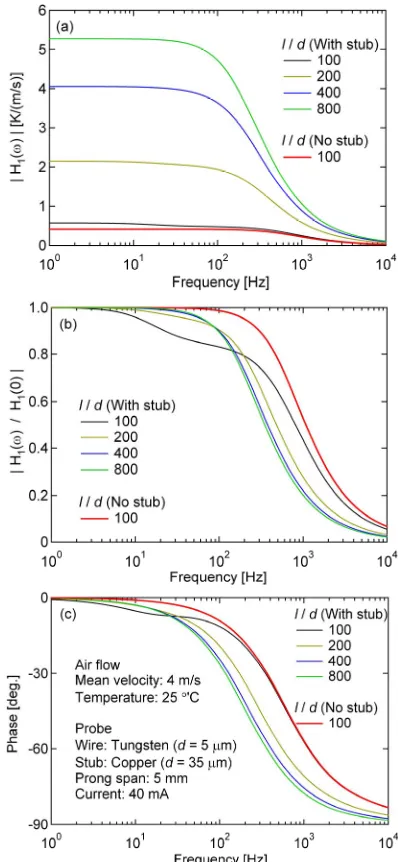
In the present analysis, the distance between the prongs (see Figure 1), air flow velocity, fluid tempera-

[image:13.595.322.521.264.695.2]

ture and the electric current to drive the CCA are set to 5 mm, 4 m/s, 25˚C and 40 mA, respectively. First, we in- vestigated the frequency response as a function of the wire length. The results are shown in Figure A1. As seen from Figure A1(a), the gain rises considerably with in-creasing wire length, since the heat loss due to conduc- tion becomes increasingly dominant as the wire length decreases. Naturally, the gain becomes lowest in the case of the shortest wire. Figures A1(b) and (c) show the Bode diagram (gain and phase) of the CCA output, where the gain is normalized by the respective values at frequency f = 0 Hz. In practice, the Bode diagram shown in Figures A1(b) and (c) can facilitate the comparison of the effects of the wire length on the response of the hot-

wire output, and we may gain a deeper understanding of the response characteristics of the CCA. As shown in

Figures A1(b) and (c), although the absolute gain at- tenuates considerably [Figure A1(a)], the frequency re- sponse improves in a high-frequency region over 200 Hz as the aspect ratio of the wire decreases. This is because the relative thermal inertia of the system consisting of the wire, stub and the prong diminishes with decreasing as- pect ratio of the wire. On the other hand, the gain in a low-frequency region smaller than 200 Hz increases, and approaches the first-order lag system. In this first-order lag system, the gain and phase take the values of

1 2