http://www.scirp.org/journal/gep ISSN Online: 2327-4344
ISSN Print: 2327-4336
Application of Flood Routing Model for
Flood Mitigation in Orashi River,
South-East Nigeria
Darlington Ogbonna, Boniface Chidi Okoro, Joachim Chinonyerem Osuagwu
Department of Civil Engineering, Federal University of Technology, Owerri, Nigeria
Abstract
The study focused on the application of Flood Routing Models for Flood Mi-tigation in Orashi River, South-East Nigeria. Flood data were collected for the study area and subjected to statistical analysis. Three flood Routingmodels were comparatively applied including Muskingum model, Level Pool model and Modified Pul’s model. Assumed routing period of 2.3 hours which helped to check excessive flood at the downstream section of the river was used. Also a dimensionless weighting factor of 0.15 was also adopted. Muskingum model and Level Pool model which represent linear relationship between measured outflow and predicted outflow for specified inflow and time change of one hour gave high and positive values of coefficients of correlations of 0.9769 and 0.9732 respectively. The Modified Pul’s model which also represents a linear relationship between measured outflow and predicted outflow for specified inflow and a time change for one hour showed the highest coefficient of corre- lation of 0.9984 and lowest standard error of 0.1749. Though, flood models of the Muskingum method and Level Pool method exhibited good correlation, their prediction differed significantly with the corresponding models of original data sets because of high standard error and thus not adequate for field application in similar rivers. A design application was carried out using the Modified Pul’s model. The values obtained for routed storage capacity was 348 m3 while the designed capacity was 354 m3. It is recommended that
dredging of the river is carried out to achieve the designed capacity. This would eliminate the risk of flooding. The results of the study will serve useful purposes in predicting flood events and design of flood control works in simi-lar basins.
Keywords
Flood Routing, Hydrologic Model, Parameter Estimation, Flood Mitigation, Channel Routing, Orashi River, Channel Design
How to cite this paper: Ogbonna, D., Okoro, B.C. and Osuagwu, J.C. (2017) Ap-plication of Flood Routing Model for Flood Mitigation in Orashi River, South-East Nige-ria. Journal of Geoscience and Environment Protection, 5, 31-42.
https://doi.org/10.4236/gep.2017.53003
Received: September 26, 2016 Accepted: February 12, 2017 Published: February 15, 2017
Copyright © 2017 by authors and Scientific Research Publishing Inc. This work is licensed under the Creative Commons Attribution International License (CC BY 4.0).
1. Introduction
When it rains or snows, some of the water generated is retained by the soil de-pending on the degree of dryness of the soil, some are absorbed by vegetation, some evaporate and the remainder, which reaches stream channels, is called runoff. Flood is an unusual accumulation of water above the ground, which is caused by high tides, heavy rainfall or rapid runoff from paved surfaces [1]. Floods occur when soil and vegetation cannot absorb all the water; water then runs off the land in quantities that cannot be carried in stream channels or re-tained in natural ponds and constructed reservoirs. About 30 percent of all pre-cipitation is runoff, and this amount may be increased by melting snow masses. Periodic floods occur naturally on many rivers, forming an area known as the flood plain. These river floods often result from heavy rain, sometimes com-bined with melting snow, which causes the rivers to overflow their banks; a flood that rises and falls rapidly with little or no advance warning is called a flash flood. Flash floods usually results from intense rainfall over a relatively small area. Coastal areas are occasionally flooded by unusually high tides induced by severe winds over ocean surfaces.
urban centers of the world and Nigeria in particular, where urbanization has dis- turbed or altered the natural process of infiltration.
The main purpose of the study was to apply flood routing models for flood mitigation in South-East Nigeria, also to compare the different methods of un-steady flow modelling using Regression approach. The study was conducted in the Orashi river watershed covering 10,000 km2 and lying between latitudes 4˚15'
and 7˚00'N and longitudes 5˚50' and 9˚00'. Natural stream flood routing was performed using different methods for solving the unsteady flow equations in order to compute stages and discharges of wave propagation. The river reach is approximately 8 km long. The channel bed is lined with mostly gravel and large boulders. The Orashi River flows past the Oguta Lake in its southwestern por-tion. It picks up volume and speed with the extra flow from Njaba River via Oguta Lake before flowing parallel to the River Niger.
Flood Routing impacts the magnitude of the peak discharge, the time of the peak discharge, depth and extent of flooding and environmental factors such as stream bank erosion, flood plain scour, sediment transport and deposition [7]. It is a technique of determining the flood hydrograph at a section of a river by uti-lizing the data of flood flow at one or more upstream sections. The hydrologic analysis of problems such as flood forecasting, flood protection, reservoir design and spillway design invariably include flood routing. In flood studies and design, the Engineer requires estimates of both the stage and discharge along a water course resulting from passage of a flood wave. The technique of flood routing is used for this purpose [8]. The hydrograph of a flood entering a Reservoir will change in shape as it emerges out of the reservoir, because certain volumes of its water is stored in the reservoir temporarily and is let off as the flood subsides. The base of the hydrograph therefore gets broadened, its peak gets reduced, and, of course, the time of peak is delayed. The extent by which the inflow hydro-graph gets modified due to the reservoir storage can be computed by a process known as flood routing [9]. Hydrograph represents how a catchment responds to rainfall [10].
2. Methodology
The data for this research were collected from National Emergency Management Agency (NEMA), FCT Abuja.
Three flood routing models were comparatively applied including Muskin-gum model, Level Pool model and Modified Pul’s model.
2.1. Muskingum Method
The graphical procedure consists of generating graphs of [XI + (1 − X)O] vs. S for different values of x, arbitrarily selected such that 0 < X < 0.5. The optimal value of x is selected as that which produces the narrowest and straightest loop graph of XI+ −
(
1 X O)
vs. S. The available data for a series of flood eventsoutflow, starting from the second time step. Then to find the change in the reach storage (S) which is the difference between the average inflow and outflow mul-tiplied by the time increment t. Secondly, the cumulative volume of reach sto-rage (Si+1), where (i ranges from one to n) can be found by adding the storage at
a previous time step (Si) to the change in storage of the next time step (Si+1).
Thirdly, a value of x is chosen from 0.1 to 1.0 and the storage (S) is plotted against the weighted flux XI+ −
(
1 X O)
. An Excel spread sheet was used toimplement the numerical procedure.
2.2. Level Pool Method
This method involved the use of Storage-Indication to route the inflow hydro-graph computed for Orashi River. Storage is nonlinear function of Q.
2.3. Modified Pul’s Method
Hydrographs of 2S O t +
∆ against outflow and a hydrograph of inflow against
time were developed. The solution to the Modified Pul’s method was accom-plished by developing a graph (or table) of [2S/Δt + O] vs. O. In order to do this, a stage-discharge-storage relationship was derived.
3. Results and Discussions
The inflow and outflow hydrographs of the river reach are tabulated in Table 1. The Attenuation which is the reduction in the peak discharge as it moves down-stream could be observed from the Table resulting in a broader flat hydrograph. The value of relative percentage attenuation computed using Equation (1) was 7.09%.
1 2
1
% Relative attenuation P – P 1001 P
Q Q
Q
= ×
(1)
where QP1 and QP2 are peakinflow and outflows (m3/s) respectively.
Using the collected data, the mean storage of the river was determined thro- ugh application of mass balance equation.
3.1. Results of the Basic Muskingum Method Application
The data in Table 1 was used to obtain the Muskingum routing parameters k and x for this river reach. The initial storage in the system was 715,000 m3. By
applying the storage calculation on a number of flood events storage loops were developed.
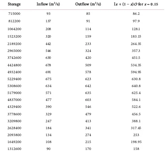
X value was taken as 0.15 since the graph of X = 0.15 gave a straight line (see
Table 1. Cumulative mean storage at X = 0.15.
Storage Inflow (m3/s) Outflow (m3/s) Ix + (1 − x)O for x = 0.15
715000 93 85 86.2
812200 137 91 97.9
1064200 208 114 128.1
1523200 320 159 183.15
2189200 442 233 264.35
2965000 546 324 357.3
3742600 630 420 451.5
4424800 678 509 534.35
4932400 691 578 594.95
5229400 675 623 630.8
5308600 634 642 640.8
5179000 571 635 625.4
4837000 477 603 584.1
4329400 390 546 522.6
3778600 329 479 456.5
3209800 247 413 388.1
2628400 184 341 317.45
2093800 134 274 253
1649200 108 215 198.95
[image:5.595.204.539.98.609.2]1312600 90 170 158
Figure 1. Plot of Weighted flux [xI + (1 − x)O] against Storage.
3.2. Determination of Outflow Values of Orashi River Using the Muskingum Routing Equation
The Muskingum routing procedure was used to route the hydrograph in Table 1. Since Δt = 1 hr, as suggested by the inflow data. However, check that with the selected Δt, parameter values meet restrictions: X < 0.5 Δt/k < 1 – X.
For this case: 0.15 < (0.5) (3600)/8205 < 1 − 0.15. Thus, OK. Proceed with
0 100 200 300 400 500 600 700
0 1 2 3 4 5 6
Ix
+
(1
-x)O
(m
3
/s
)
routing, by obtaining C1, C2, and C3 using Equations (7) - (9) respectively.
Since K = 2.3 hours, time interval = 1 hours, and X = 0.15 Values of K, t, and X into the Equations (7) - (9)
Applying Muskingum routing Equation:
1 1 2 1 3
i i i i
O+ =C I +C I+ +C O (2)
2 2
I O S=K +
(3)
But we also have
1 2 1 2 2 1
2 2
I I O O S S
t
+ − + = −
∆ (4)
Note: Δt = 1 hour = 3600 sec.
(
1 ?)
S =K XI + X O (5)
where S is storage (m3), K is the travel time in seconds between the two channel
sections, O (m3/s) is the outflow (m3/s), I is the inflow (m3/s), and x is a dime-
nsion less factor between 0.0 and 0.5 that weights the influence of the inflow and outflow hydrograph to thestorage within the reach.
1 1 2 1 3
i i i i
O+ =C I +C I+ +C O (6)
where:
(
)
1 2 2 1 t KX CK X t
∆ − =
− + ∆ (7)
(
)
2 2 2 1 t KX CK X t
∆ + =
− + ∆ (8)
(
)
(
)
3
2 1
2 1
K X t
C
K X t
− − ∆ =
− + ∆ (9)
C1, C2, and C3 are also known as Courant factors.
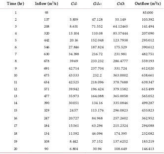
The results using Muskingnum method to determine the outflow data are presented in Table 2.
3.3. Level Pool Routing Method
This hydrograph flows into a reservoir whose storage and discharge characteris-tics are as presented in Table 3. The initial storage in the system is 0 m3 and the
initial outflow is 85 m3/s.
For a given set of conditions, the outflow is unique, independent of how that stage is achieved. The peak outflow occurs when the outflow hydrograph inter-sects the inflow hydrograph.
Hydrographs of 2S O t +
∆ against outflow and inflow against time were pre-
pared. The concept involved development of the function
( )
2SO f O
t + =
∆
And solving sequentially for every time step.
The following data were relevant in preparing the Table;
• Elevation vs. Outflow discharge and hence storage vs. outflow discharge. • Inflow hydrograph
• Initial values of inflow, outflow O, and storage S at time t = 0.
3.4. Modified Pul’s Method
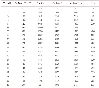
The results using Pul’s method to determine the outflow data for the River are presented in Table 4.
Again, the general continuity equation was adopted. However, in this case, a finite difference form of the continuity equation was used. A graph of [2S/Δt + O] vs. O was derived. In order to do this, a stage-discharge-storage relationship was developed and plotted as a curve. The basic assumption is that a unique and single-valued stage-storage-outflow relationship exists for each reach.
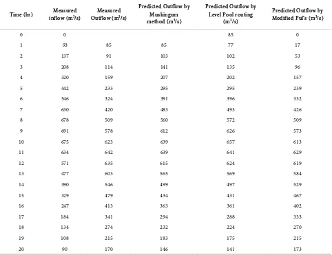
A Summary of measured inflows/outflows and predicted outflows from the three models are presented in Table 5.
The results indicate that Level pool method gave highest value of predicted peak outflow (657 m3/s) while the modified Pul’s method gave the least value
(629 m3/s). The derived Regression models are presented in Table 6.
The weighing factor, X value was taken as 0.15.
[image:7.595.207.539.424.736.2]Based on the value of X, the storage constant K which indicate the routing period was then computed from the slope of the graph; k = slope of graph = 8205 sec; which was taken as 2.3 hours approximately.
Table 2. Prediction of outflow data of Orashi using Muskingum method.
Time (hr) Inflow (m3/s) C1Ii C2Ii+1 C3Oi Outflow (m3/s)
1 93 85.000
2 137 5.859 47.128 55.149 103.392
3 208 8.631 71.552 64.12465 141.494
4 320 13.104 110.08 85.57444 207.090
5 442 20.16 152.048 123.7938 295.012
6 546 27.846 187.824 175.529 390.612
7 630 34.398 216.72 231.981 482.751
8 678 39.69 233.232 286.4777 559.193
9 691 42.714 237.704 331.724 612.020
10 675 43.533 232.2 363.0002 638.661
11 634 42.525 218.096 378.7688 639.347
12 571 39.942 196.424 379.1582 615.499
13 477 35.973 164.088 365.0058 565.052
14 390 30.051 134.16 335.0846 499.287
15 329 24.57 113.176 296.0823 433.823
16 247 20.727 84.968 257.2602 362.952
17 184 15.561 63.296 215.2324 294.088
18 134 11.592 46.096 174.395 232.082
19 108 8.442 37.152 137.6252 183.219
Table 3. Orashi River results of outflows for various inflows using Level Pool method.
Time(hr) Inflow (m3/s) Outflow (m3/s) I i + I(i+1)
(m3/s)
2S O t+ ∆ (m3/s)
2 i
i
S O t + ∆
( 1) 1
2 i
i
S O t
+ +
+
∆ O (m3/s)
1 93 85 93 482 387.6 405.2 77.3
2 137 91 230 542 501.9 617.6 101.6
3 208 114 345 705 734.7 846.9 135.3
4 320 159 528 1005 1045.4 1262.7 201.9
5 442 233 762 1449 1380.3 1807.4 295.4
6 546 324 988 1971 1706.8 2368.3 396.2
7 630 420 1176 2499 1981.3 2882.8 492.9
8 678 509 1308 2967 2173.6 3289.3 572.3
9 691 578 1369 3318 2276.1 3542.6 626.1
10 675 623 1366 3528 2276.6 3642.1 657.3
11 634 642 1309 3591 2229.2 3585.6 641.5
12 571 635 1205 3512 2042.7 3434.2 623.8
13 477 603 1048 3290 1812.3 3090.7 569.5
14 390 546 867 2951 1583.9 2679.3 497.2
15 329 479 719 2578 1333.4 2302.9 431.4
16 247 413 576 2196 1079.8 1909.4 360.7
17 184 341 431 1801 862.1 1510.8 287.5
18 134 274 318 1437 682.4 1180.1 224.4
19 108 215 242 1131 549.5 924.4 174.9
20 90 170 198 899 −282.6 747.5 141.3
Table 4. Results of the Modified Pul’s method for Orashi River.
Time (h) Inflow, I (m3/s) In + In+1 2Sn/dt − On 2Sn/t + On+1 On+1
1 93 230 59 93 17
2 137 345 183 289 53
3 208 528 331 523 96
4 320 762 545 860 157
5 442 988 829 1307 239
6 546 1176 1153 1817 332
7 630 1308 1477 2329 426
8 678 1369 1767 2785 509
9 691 1366 1989 3136 573
10 675 1309 2128 3355 613
11 634 1205 2180 3437 629
12 571 1048 2147 3385 619
13 477 867 2027 3195 584
14 390 719 1835 2894 529
15 329 576 1620 2554 467
16 247 431 1392 2196 402
17 184 318 1157 1823 333
18 134 242 935 1475 270
19 108 198 747 1177 215
[image:8.595.204.539.440.738.2]Table 5. Summary of Orashi River predicted outflow by Muskingum, Level Pool Routing and Modified Pul’s methods.
Time (hr) Measured inflow (m3/s)
Measured Outflow (m3/s)
Predicted Outflow by Muskingum method (m3/s)
Predicted Outflow by Level Pool routing
(m3/s)
Predicted Outflow by Modified Pul’s (m3/s)
0 0 85 0
1 93 85 85 77 17
2 137 91 103 102 53
3 208 114 141 135 96
4 320 159 207 202 157
5 442 233 295 295 239
6 546 324 391 396 332
7 630 420 483 493 426
8 678 509 560 572 509
9 691 578 612 626 573
10 675 623 639 657 613
11 634 642 639 641 629
12 571 635 615 624 619
13 477 603 565 569 584
14 390 546 499 497 529
15 329 479 434 431 467
16 247 413 363 361 402
17 184 341 294 288 333
18 134 274 232 224 270
19 108 215 183 175 215
20 90 170 146 141 173
Table 6. Summary of predicted/measured outflow models for Orashi River.
S/N Method Regression equation coefficient (cc) Correlation Standard error
1 Muskingum Method Y = 0.964X + 14.67 0.9769 0.4262
2 Level Pool method Y = 0.993X + 5.159 0.9732 0.46499
3 Modified Pul’s method Y = 1.019X − 17.83 0.9984 0.1749
This indicates the released period that will allow for effective storage and prevent excessive flood at the downstream section of the river.
The developed parameter estimation methodology was applied to determine the K, and X values for flow routing corresponding to the river inflow-outflow. The value S of K and X was used to route the flood using three different me-thods.
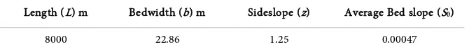
[image:9.595.207.539.497.584.2]3.5. Design Application of the Modified Pul’s Model to Orashi River
The characteristics of Orashi River Channel are presented in Table 7.
(
–)
Storage= I O ∆t
where I = Inflow (m3/s), O = Outflow (m3/s), Δt = time (s)
Inflow (I) and outflow (O) are functions of time (t), and the storage (S) is a function of the water surface elevation (H) which changes with time (t).
UsingY =1.019x−17.83 [11] (10)
where, Y = predicted outflow (m3/s) of Orashi river, x = measured outflow
(m3/s) of Orashi river.
The values of measured outflow are shown in Table 5.
Since Inflow is greater than outflow, there will be no flood. A channel that can store 1.26 × 10⁶ m3 is recommended.
The river reach is approximately 8 km long and a sharp crested weir is located 3.93 km from the upstream section of the river. The channel bed is lined with mostly gravel andlarge boulders.
The Orashi River has a trapezoidal cross-section with no recent floodplain
[12]. Due to the weir transition downstream the river, a cross-section which is locatedat the upstream end is only considered in modelling.
The nature of the flow in the river Orashi is non-uniform, gradually varied unsteady flow. To determine the regime of flow upstream of the channel, Equa-tion 11wass used to calculate the Froude Number.
1
V Fr
gy
= (11)
(
)
0 0 0
V =Q b+zy y [13] (12)
where, V is the average velocity in (m/s) which can be defined from Equation (13), y1 is depth of flow upstream in m and g = 9.81 m/s2.
In channel routing where a non-uniform flow is the case, the average velocity can bedetermined using a reference discharge and the channel cross-sectional area as in Equation (12). To determine the normal depth y0, a reference discharge
is selected for a maximumflood event and can be calculated from Equation (13) Reference discharge, Q0:
(
)
(
)
0 b 0.5 p b
Q =Q + Q −Q (13)
where Qb = Minimum discharge in (m3/s), Qp = Peak discharge in (m3/s)
3 3
69 , 636
b p
Q = m s Q = m s
(
)
30 69 [0.5 636 69 ] 354
Q = + − = m s
[image:10.595.207.542.693.730.2]Therefore, reference discharge is 354 m3/s.
Table 7. Channel parameters of orashi river.
Length (L) m Bedwidth (b) m Sideslope (z) Average Bed slope (S0)
With the known values of reference discharge (Q0), Manning roughness
coefficient (n), Channel bed width and bottom slope, the value of Φ can be determined from Equation (13)
(
)
83 120 0
Q n b s
∅ =
(14)
(
) (
) (
8)
0.5 3
354 0.04 22.86 0.00047
∅ = ×
2
0.16m s
∅ =
Upon consulting Table 7 with the above value ( 2
0.16m s
∅ = ) and with z =
1.25 the value of y b0 ≈0.54, hence, y0 = 12.34 m, where, b = 22.86 m.
The area of flow A, can then be obtained from Equation (14) A= [b + (zy0)]y0 × 15
A = [22.86 + 1.25(12.34)] × 12.34 A = 472.44 m2
Hence, Velocity, V =
(
Referencedischarge)
AreaV=354 472.44
V=0.749m s
Therefore,
0.14 1
Fr= <
This indicates that the channel has a mild slope and the flow is characterised as gradually varied subcritical flow. The wave celerity (c) can be obtained from the relationship
16
c=βV
where β is assumed to be 0.5 and velocity, V = 0.749
C 0.5 0.749= × =0.375m s
Therefore, storage = area × velocity × time = 1272700.8 m3.
4. Conclusions
Based on the result obtained from the Orashi flood routing studies, the following conclusions can be made.
• Three sets of mathematical modeling of Orashi river flood routing based on
regression-correlation approach were analyzed namely: 1) Muskingum routing model
2) Level Pool routing model 3) Modified Pul’s model
• In the Modified Pul’s model, very high and positive values of coefficient of
correlation of 0.9984, as well as a standard error of 0.1749 was obtained. This model provided the best-fit curve for the field data.
• Plots of Modified Pul’s model are in conformity with the field data. They
equally agree with literature as follows:
2) During the determination of routing parameter, the courant factor did not exceed one, using Modified method.
Since Modified Pul’s method gave the most accurate result of predicted out-flow, the method should be adopted as a model for flood mitigation in Orashi River. The design capacity based on this model is 354 m3 which is higher than
the routed storage capacity of 348 m3. To guarantee a check against flooding, it is
recommended that dredging is carried out to achieve the designed capacity.
References
[1] Kulandaiswamy, V.C. (2006) A Note on Muskingum Method of Flood Routing. Journal of Hydrology, 4, 273-276.https://doi.org/10.1016/0022-1694(66)90085-0 [2] NEST (1991) Flood Hazard Assessment, Management and Mitigation Measures.
Nigerian Environmental Study/Action Team NEST Publication, Ibadan, 67-70. [3] Pitt, P.H. (2007) Lessons from 2007 Floods. Pitt Review Report, Lancaster. [4] Smith, K. (2006) Environmental Hazards. Routledge, London, 301-314.
[5] Akin, T. (2009) Strategies for Combating Urban Flooding in a Developing Nation: A Case Study from Ondo, Nigeria.Environmentalist, 14, 57-62.
[6] NEST (1991) National Environmental Survey/Action Flood Report.
[7] King, L. (2014) Flood Routing. National Engineering Handbook. US Department of Agriculture. Part 630 chap 17.
[8] Chadwick, A. and Morfeit, J. (1993) Hydraulics in Civil and Environmental Engi-neering. E & F N Spon, London, p. 317.
[9] Garg, S.K. (2008) Irrigation Engineering and Hydraulic Structures. Khanna Pub-lishers, Delhi, p. 937.
[10] Han, D. (2010) Concise Hydrology. Bookboon.com Ltd., London, 119-124.
[11] Ogbonna, O. (2015) Application of Flood Routing Model for Flood Mitigation in Orashi River, South-East Nigeria. PhD Thesis, Federal University of Technology, Owerri. (Unpublished)
[12] NEMA (2012) Evaluation of Flood Hazards. Prepared by EnvironmentalImpact Assessment Department, 13-16.
Submit or recommend next manuscript to SCIRP and we will provide best service for you:
Accepting pre-submission inquiries through Email, Facebook, LinkedIn, Twitter, etc. A wide selection of journals (inclusive of 9 subjects, more than 200 journals)
Providing 24-hour high-quality service User-friendly online submission system Fair and swift peer-review system
Efficient typesetting and proofreading procedure
Display of the result of downloads and visits, as well as the number of cited articles Maximum dissemination of your research work
Submit your manuscript at: http://papersubmission.scirp.org/