Parametric Optimization of Solar Parabolic Collectors Using AHP TOPSIS

(1)

© 2017, IRJET | Impact Factor value: 5.181 | ISO 9001:2008 Certified Journal

| Page 270

Parametric Optimization of Solar Parabolic Collectors Using

AHP-TOPSIS

J Ravi Kumar

1

_{, K Dharma reddy}

2

_{, P Venkataramaiah}

3

1

_{PG Scholar, Dept. of Mechanical Engineering, Sri Venkateswara University, Tirupati, A.P., India.}

2

_{Assistant Professor, Dept. of Mechanical Engineering, Sri Venkateswara University, Tirupati, A.P., India.}

3

_{Professor, Dept. of Mechanical Engineering, Sri Venkateswara University, Tirupati, A.P., India.}

---*---Abstract - In the present work the behavior of linear solar**

parabolic Collector is studied. An experimental design is prepared based on the considered parabolic collector parameters such as Temperature, Discharge and Period of Sun Incidence (POI). The copper alloy c101 tube and aluminum alloy 1199 are used in experimental setup as absorbers. Copper alloy c101 tube has composition of Copper(99.998%), Antimony (0.1ppm), Arsenic(0.1ppm), Bisumasu (0.1ppm), Cadmium (<0.1ppm), Iron (1ppm), Lead (1ppm), Manganese (<=0.1ppm), Nickel (0.5ppm) and Aluminium alloy1199 has aluminium (99.98%), copper (0.006%), gallium (0.005%), iron (0.005%), titanium(0.002%), magnesium (0.006%) and the reflective surfaces are considered at two levels, one is Glass mirror and other is polished aluminum. Present work is focused on improvement of temperature of working fluid (water) and discharge of fluid, which influenced by parameters such as absorber tube materials, reflective sheet materials, time duration. The experiments are conducted according to the Taguchi design on the solar parabolic collector. This data is analyzed using AHP-TOPSIS and optimal parameter combination has been identified.

Key Words

: 1)Parabolic Shaped Structure, 2)

Supporting legs, 3) Reflective Surfaces, 4) Heat

collecting element(Absorber), 5) Auto Tracking

System, 6) Piping system and Storage tank.

1. INTRODUCTION

The powerful presence of the sun is hard to ignore in one’s everyday life: indeed, the majority of life on Earth could not exist without its vast output of radiant energy. At any given moment, the Earth’s upper atmosphere receives solar radiation amounting to 174 PW (Peta Watts) of power. As shown in Figure 1.2, about 55% of this reaches the Earth’s surface and is either absorbed or reflected by land and oceans. With such a vast amount of solar energy available, humanity could meet its demands by harnessing just a small fraction of this. Indeed, the total annual solar radiation falling on the Earth is more than 7500 times greater than the world’s total annual primary energy consumption (WEC 2007). Furthermore, unlike fossil fuels, solar energy will continue to be available for billions of years.

1.1 Introduction of Solar Thermal systems

Concentrating solar technologies, such as the parabolic dish, compound parabolic collector and parabolic trough can operate at high temperatures and are used to supply industrial process heat, off-grid electricity and bulk electrical power. In a parabolic trough solar collector, or PTSC, the reflective profile focuses sunlight on a linear heat collecting element (HCE) through which a heat transfer fluid is pumped. The fluid captures solar energy in the form of heat that can then be used in a variety of applications.

1.2 Experimental Setup

(a) The experimental setup consists of the following components:

1)Parabolic Shaped Structure, 2) Supporting legs, 3) Reflective Surfaces, 4) Heat collecting element(Absorber), 5) Auto Tracking System, 6) Piping system and Storage tank.

The whole experimental setup is placed on the top of the buildings. All the components are assembled to form the entire setup. The entire set is placed in the N_S direction to face the axis of the parabolic trough towards east.

(b) Plan of investigation: It is planned that the experiments are conducted according to the L36 array with respect of factors and levels of problem.

Table2.: Process parameters and their levels

S.

No

Process Parameters

Level 1 Level 1 Level 1

1 Reflectivity Polished Aluminum (AP)

Glass Mirror (GM)

-

2 Absorptivity Copper Alloy C101 tube

Aluminum Alloy 1199 tube

-

3 Period of sun

incidence (POI)

10.00AM-12.00PM

12.00PM-2.00PM

(2)

© 2017, IRJET | Impact Factor value: 5.181 | ISO 9001:2008 Certified Journal

| Page 271

Fig-1.Experimental Setup

2. EXPERIMENTAL WORK

The experiments were conducted for several days on the solar parabolic trough by changing the reflective and absorber materials. After absorbing sufficient radiation, the water in the absorber tube gets heated and its density decreases. Due to the differential, and the end of the absorber tube is closed the natural convection in counter flow direction has occurred .at each experiment the temperature is noted at the surface of the absorber and bottom of the water tank ,the water in storage tank is heated by the natural convection.

Table2.1: Experimental results and response data

POI Absor

-ber Tube

Refle

-ctor Output Temp (°C)

Dischar -ge (lit/hr)

Thermal efficiency (%)

10

a.m-12p.m Cu alloy GM 60.6 19 89.37

12a.m-2p.m Cu alloy GM 75.3 16 135

2p.m-4p.m Cu alloy GM 68.1 18.5 112.5

10a.m-12p.m Cu alloy GM 61.3 18.3 91.6

12p.m-2p.m Cu alloy GM 78.5 15 145

2p.m-4p.m Cu alloy GM 65.5 17 104.68

10a.m-12p.m Cu alloy GM 59 19.1 84.37

12p.m-2p.m Cu alloy GM 77 15.5 140.6

2p.m-4p.m Cu alloy GM 65.2 18 103.7

10a.m-12p.m Cu alloy Al Sheet 51 19.4 59.37

12p.m-2p.m Cu alloy Al Sheet 65.3 18.7 104.06

10a.m-12p.m Cu alloy Al Sheet 50.4 19 57.5

10a.m-12p.m Cu alloy Al Sheet 49.3 19.2 54.06

12p.m-2p.m Cu alloy Al Sheet 66 18.4 106.25

2p.m-4p.m Cu alloy Al Sheet 59.2 18.6 85

10a.m-12p.m Al alloy GM 50 19.3 56.25

12p.m-2p.m Al alloy GM 68.2 18.5 113.12

2p.m-4p.m Al alloy GM 59.2 19 85

10a.m-12p.m Al alloy GM 49.2 19.1 54.06

12p.m-2p.m Al alloy GM 67.5 18.7 110.09

2p.m-4p.m Al alloy GM 58.2 19 81.8

10a.m-12p.m Al alloy GM 51.2 19.2 60

12p.m-2p.m Al alloy GM 69.3 18 116.56

2p.m-4p.m Al alloy GM 59.4 18.7 85

10a.m-12p.m Al alloy Al Sheet 46.2 19.6 44.37

12p.m-2p.m Al alloy Al Sheet 58.1 19.1 81.56

12p.m-2p.m Al alloy Al Sheet 57.6 19 80

2p.m-4p.m Al alloy Al Sheet 48.2 19.6 56

3. EVALUATION OF WEIGHTAGE FOR RESPONSES

USING IN AHP

(3)

© 2017, IRJET | Impact Factor value: 5.181 | ISO 9001:2008 Certified Journal

| Page 272

Step I

Specify the set of criteria for evaluating the weights and tabulated in Table3.1

Temperature Efficiency Discharge

Temperature EP Not

BEtMP

Not MP

Efficiency BEtMP EP Not

BEtMP

Discharge MP BEtMP EP

Step II

The criterion is compared with each other in order to determine the relative importance of each factor to accomplish the overall objective. The importance of each factor is represented on the left (row) relative to the importance of the factor on top (column) of the matrix. Thereby, consider the higher value which means the factors on the left is relatively more important than the factor on the top and compute the priorities or weights of the criteria based on this information and is tabulated as in Table

Table3.2: Pair wise comparison matrix Tem

p Therma-l Efficien

cy

Discha

r-ge ValueEigen s (EV)

Weighta g-es (EV/3.36

7)

Temp 1 1/2 1/3 0.550

2 0.1633 Efficien

cy 2 1 1/2 1 0.2969

Dischar

ge 3 2 1 1.8171 0.5396

Total 6 3.5 1.83 3.367

3

λmax 3.007

Step III

Compute Eigen vectors for each matrix by approximation of priorities using geometric mean method. This is done by multiplying the elements in each row and taking their nth root and these values are shown below. Where n is number of criteria.

 Eigen vector or value for Temperature

EVtemp=

 For Efficiency

EV Effi=  For Discharge

EV Dis= Step IV

Sum of each column is then multiplied with corresponding Priority vector. Sum of column one with Priority vector of component one and so on and sum of product is called Principal Eigen vector.

λ max = *Pvi λ max = 3.006

Step V

Consistency index is calculated using the equation C. I = (λmax - n)/n – 1

C.I= (λmax-n)/(n-1) = (3.006-3)/3-1 = 0.0032 Then calculation of consistency ratio (CR)

In this case R.I is 0.58 as the size of matrix is three (Table 4.2). The value of CR should be around 10% to be acceptable.

C.R = (C.I/R.I) = (0.0032 /0.58) = 0.055

Hence the C.R is less than 10%; therefore the pair wise comparison matrix is acceptable and the weightage obtained for output responses as follows.

Weightages:

Temperature =0.1633

Thermal Efficiency =0.2969 Discharge =0.5396

4. SELECTION OF OPTIMAL PROCESS PARAMETERS COMBINATION USING TOPSIS METHOD

TOPSIS method is used to determine the optimum parameter combination by analyzing the experimental data.

Step1: The first step is to formulate decision matrix with ‘m’ alternatives and ‘n’ attributes are shown in table 3.1.

(4)

© 2017, IRJET | Impact Factor value: 5.181 | ISO 9001:2008 Certified Journal

| Page 273

rij= ……….(1)

𝑉𝑖𝑗 = 𝑊𝑖 × 𝑟𝑖𝑗……….…….(2)

Si+ = ……… (3)

Si- = ………..… (4) Table4.1: Normalization Matrix

Step 4: After obtaining weighted normalized matrix, Positive separation ideal solution (PIS) and negative separation ideal solution (NIS) are determined. Using Equations 3 and 4. These ideal solutions are as follows.

From weighted normalized decision-making matrix, the positive separation ideal solution V+ _{obtained as}

V+_{= {0.036, 0.052, 0.143}}

From weighted normalized decision-making matrix, the negative separation ideal solution V-_{obtained as}

V-_{= {0.019, 0.039, 0.036}}

Step 5: The separation of each alternative from positives separation ideal solution (PSIS) and negative separation NORMALISATION MATRIX

s.no Output

Temp Discharge Efficiency

1 0.1702 0.1701 0.1695

2 0.2116 0.1432 0.2561

3 0.1913 0.1655 0.2134

4 0.1722 0.1638 0.1738

5 0.2205 0.1342 0.2751

6 0.1840 0.1521 0.1986

7 0.1658 0.1709 0.1601

8 0.2163 0.1387 0.2657

9 0.1832 0.1611 0.1967

10 0.1433 0.1736 0.1126

11 0.1835 0.1673 0.1974

12 0.1632 0.1709 0.1547

13 0.1416 0.17007 0.1091

14 0.1747 0.1682 0.1791

15 0.1576 0.1539 0.1429

16 0.1385 0.1718 0.1025

17 0.1854 0.1647 0.2016

18 0.1663 0.1664 0.1612

19 0.1405 0.1727 0.1067

20 0.1916 0.1655 0.2146

21 0.1663 0.17007 0.1612

22 0.1382 0.1709 0.1025

23 0.1896 0.1673 0.2088

24 0.1635 0.17007 0.1552

25 0.1438 0.1718 0.1138

26 0.1947 0.1611 0.2211

27 0.1669 0.1673 0.1612

28 0.1298 0.1754 0.0841

29 0.1632 0.1709 0.1547

30 0.1382 0.1736 0.1018

31 0.1275 0.1763 0.0794

32 0.1618 0.17007 0.1518

33 0.1354 0.1754 0.1062

34 0.1216 0.1772 0.0670

35 0.1551 0.1718 0.1375

36 0.1306 0.1736 0.0859

WEIGHTED NORMALSED MATRIX

s.no

Output

Temp

Discharg

e

Efficienc

y

1

0.027

0.051

0.091

2

0.034

0.042

0.138

3

0.031

0.049

0.115

4

0.028

0.048

0.093

5

0.036

0.039

0.148

6

0.031

0.045

0.107

7

0.027

0.051

0.086

8

0.035

0.041

0.143

9

0.029

0.047

0.106

10

0.023

0.051

0.061

11

0.029

0.049

0.106

12

0.026

0.051

0.083

13

0.023

0.051

0.058

14

0.028

0.049

0.096

15

0.025

0.045

0.077

16

0.022

0.051

0.055

17

0.031

0.048

0.108

18

0.027

0.049

0.087

19

0.022

0.051

0.057

20

0.031

0.049

0.115

21

0.027

0.051

0.087

22

0.022

0.051

0.055

23

0.030

0.049

0.112

24

0.026

0.051

0.083

25

0.023

0.051

0.061

26

0.031

0.047

0.119

27

0.027

0.049

0.087

28

0.021

0.052

0.045

29

0.026

0.050

0.083

30

0.022

0.051

0.054

31

0.020

0.052

0.042

32

0.026

0.050

0.081

33

0.022

0.052

0.057

34

0.019

0.052

0.036

35

0.025

0.051

0.074

(5)

| Page 274

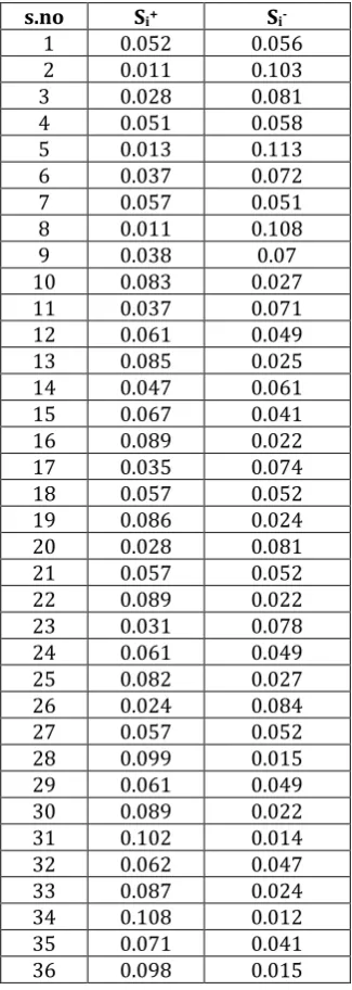
ideal solution (NSIS) are calculated using the equation as in

[image:5.595.54.217.141.598.2]

the Table 4.3

Table 4.3: Positive and Negative Separation ideal solution

Step 6: The closeness co-efficient (Table 4.4) of each

alternative is CCi =

Table 4.4: Closeness coefficient

Step 7: Rank the preference order based on their largest relative closeness co-efficient. It is observed from the Table 4.4, for the higher closeness coefficient is obtained for 8th_{experimental run. Hence the best parameter} combinations of experimental 8th_{run are in the following.} Best combination of parameter

 Period of incidence : 12.00 p.m. – 2.00 p.m.  Absorber Tube : Copper alloy c101  Reflector : Glass Mirror Best Output Responses for best combination of reflector and absorber tube

 Temperature : 77°C  Discharge : 15.5 lit/hr.  Thermal Efficiency : 140.6%

s.no Si+ S

1 0.052 0.056 2 0.011 0.103

3 0.028 0.081

4 0.051 0.058

5 0.013 0.113

6 0.037 0.072

7 0.057 0.051

8 0.011 0.108

9 0.038 0.07

10 0.083 0.027

11 0.037 0.071

12 0.061 0.049

13 0.085 0.025

14 0.047 0.061

15 0.067 0.041

16 0.089 0.022

17 0.035 0.074

18 0.057 0.052

19 0.086 0.024

20 0.028 0.081

21 0.057 0.052

22 0.089 0.022

23 0.031 0.078

24 0.061 0.049

25 0.082 0.027

26 0.024 0.084

27 0.057 0.052

28 0.099 0.015

29 0.061 0.049

30 0.089 0.022

31 0.102 0.014

32 0.062 0.047

33 0.087 0.024

34 0.108 0.012

35 0.071 0.041

36 0.098 0.015

s.no CCI RANK

1 0.521 14

2 0.901 2

3 0.736 6

4 0.539 13

5 0.892 3

6 0.657 9

7 0.473 18

8 0.904 1

9 0.652 11

10 0.248 26

11 0.657 10

12 0.447 20

13 0.228 27

14 0.566 12

15 0.382 23

16 0.201 30

17 0.677 8

18 0.478 17

19 0.221 28

20 0.742 5

21 0.479 15

22 0.201 31

23 0.714 7

24 0.449 19

25 0.252 25

26 0.772 4

27 0.478 16

28 0.135 34

29 0.447 21

30 0.201 32

31 0.123 35

32 0.432 22

33 0.221 29

34 0.105 36

35 0.364 24

(6)

| Page 275

Conclusions

The following conclusions are drawn from the results.  In the present work, the behaviour of linear solar

parabolic Collector for cooking system is studied and analysed using Mathematical models.  Finally experimental response data is analysed

using AHP-TOPSIS and optimum parameters levels have been identified.

 Among the combination of different reflector and absorber, glass mirror and copper alloy c101 tube combination is given best results for obtaining maximum temperature and discharge, thermal efficiency.

References

[1] A. Kahrobaian and H. Malekmohammadi (2008): Energy optimization Applied to Linear Parabolic Solar collectors. Journal of faculty of engineering, Vol.42.No.1 2008 PP-131-144

[2] Aneirson Francisco and da silva (2013): Multi-choice mixed integer goal programming optimization for real problems in a sugar and ethanol milling company, Applied Mathematical Modeling, 37(2013) 6146-6162. [3] Delfin Silio Salcines, Carlos Renedo Estebanez (2009):

Simulation of solar domestic water heating system, with different collector efficiencies and different volume storage tanks.

[4] Fernandez-Garcia, E.Zarza (2010) “Parabolic solar through collectors and their applications” Elsevier journal of Renewable energy, Vol.14, pp.1695–1721 [5] Sairam, P. Mohan Reddy and P. Venkataramaiah

Parametric Optimization of Solar Parabolic Collectors Using AHP TOPSIS

© 2017, IRJET | Impact Factor value: 5.181 | ISO 9001:2008 Certified Journal

| Page 270