Evaluation of Traffic Characteristics: a Case Study on NH 12, Near Barkatullah University, Bhopal (M P )

(1)

Evaluation of Traffic Characteristics: a Case Study on NH-12,

Near Barkatullah University, Bhopal (M.P.)

Mrityunjay Singh

1

_{, Dr. Y P Joshi}

2

_,

1

_{Student – M.E. Civil (transportation)}

_{Department of civil engineering S.A.T.I. Vidisha (M.P), India}

2

_{Professor, Department of civil engineering S.A.T.I. Vidisha (M.P), India}

---*---Abstract -**

Speed is a life and death transportation

deliberation because it relates to safety, time, comfort, convenience, and economics. Spot speed studies are used to determine the speed distribution of a traffic stream at a certain location. The data assembled in spot speed studies are used to determine vehicle speed percentiles, which are useful in making many speed decisions. The intention of spot speed studies are to record speed characteristics under prevailing traffic conditions at a specific site along a roadway. Because traffic engineering demands the collection and analysis of immense amount of data for performing all types of traffic studies, it follows that spot speed study is also a vital element in traffic engineering. Now a day’s managing traffic within our communities is a growing task for traffic engineers. As traffic volume increases and public financial resources decrease, targeting improvement projects to predict growth patterns is censorious. This paper represents traffic condition of Barkatullah university route Bhopal NH-12 Madhya Pradesh.

Key Words

:

Spot speed; Mean Speed, Flow, 85th Speed,

Cumulative Frequency, Vehicle Speed, and Vehicle Volume

1. INTRODUCTION

Speed plays a life and death role in evaluating the safety of road network. Speed by definition is the distance travelled in unit time. The typical unit of speed is kilometer per hour (kmph) or miles per hour (mph). Basically there are two types of speed; time mean speed and space – mean speed. Space mean speed is the length of a road section divided by the average travel time of several vehicles over this specific section. The time mean speed (spot) speed is the average spot speed of several vehicles measured at a given spot.

1.1

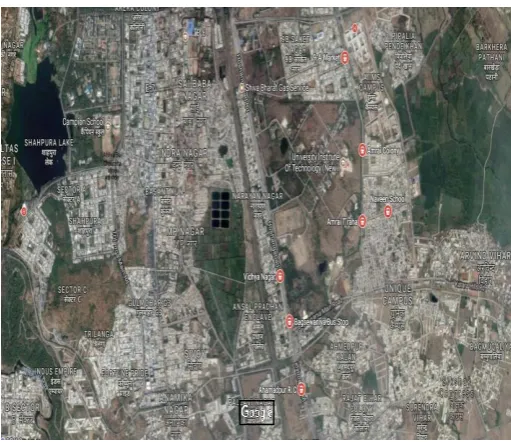
Area of study

Area of study is Hoshangabad road, near Barkatullah University, Bhopal; Madhya Pradesh is a NH-12 which connects Jaipur in Rajasthan with Jabalpur in Madhya Pradesh. The total length of NH-12 runs to 612 km starting from national highway7 in Jabalpur it runs northwards and ends at Jaipur at NH-11.

2.

LITRATURE REVIEW

A. Introduction

A spot speed study is made by measuring the individual speeds of a sample of the vehicles passing a given point (spot) on a street or highway. These individual speeds are used to estimate the speed distribution of the entire traffic Stream at that location under the conditions prevailing at the time of study.

B. Uses of Spot Speed Data

The result of spot speed studies are used for many different purposes by traffic engineers, including:

1. Establishing the effectiveness of new or existing speed limits or enforcement practices.

2. Determining appropriate speed limits for application. 3. Establishing speed trends at the local, state, and national level to assess the effectiveness of national policy on speed limits and enforcement

4. Specific design application determining appropriate sight distances, relationships, between speed and highway alignment, and speed performance with respect to steepness and length of grades.

5. Specific control applications for the timing of “yellow” and “all red” intervals for traffic signals, proper placement of signs, and development of appropriate signal progressions. 6. Investigation of high-accident locations at which speed is suspected to be a contributing cause to the accident experience.

C. Data Requirements

(2)

[image:2.595.34.298.75.334.2]

D. Determine an Appropriate Selection Strategy

Except for studies conducted under low-volume conditions, it is impossible to obtain a radar measurement for every vehicle. For Every vehicle peak flow analysis, speeds are measured during the peak period. For assessing general speed trends or for setting speed limits, off-peak measurements are more appropriate.

The selection of the target vehicle that represents the vehicle population under study is also important. A good question to ask is, “What type or types of vehicles are of concern—cars, trucks, buses, or others?” Typically cars, station wagons, pickup and panel trucks, and motorcycles are classified as passenger cars. Other trucks and buses are classified as trucks. School buses and farm equipment may be recorded separately. When the target vehicle is defined, a selection strategy is developed to provide a random sample. A random sample will reduce the tendency to select the vehicles that stand out. For example, the observer could obtain a speed reading from every fourth vehicle or every tenth vehicle.

3 METHODOLOGY

A. Introduction

The objective of this study is to get traffic characteristics from Mandideep route Bhopal NH-12 Madhya Pradesh include spot speed and flow.

This study are used to determine the level of service for streets

Document congestion and quantify the need for street improvements and also for a variety of purposes. For a spot speed study at a selected location, a sample size of at least 50 and preferably 100 vehicles is usually obtained (Ewing

1999). Traffic counts during a Monday morning or a Friday peak period may show exceptionally high volumes and are not normally used in the analysis; therefore, counts are usually conducted on a Tuesday, Wednesday, and Thursday. Spot speed data are gathered using one of three methods: (1) Stopwatch method,

(2) Radar meter method,

(3) Pneumatic road tube method.

The stopwatch method is the least expensive and least accurate of the methods.

Figure 2 .map of observation point

B. INSTRUMENT

Counter

A Counter meter is a commonly used to take the number. In this method, the observer stay at the point of interest and count the vehicles with the help of hand tallies using counter meter (Fig. 3).

Radar Meter

A radar meter is a commonly used device for directly measuring speeds in spot speed studies (Fig. 4 ). This device may be handheld, mounted in a vehicle, or mounted on a tripod. The effective measuring distance for radar meters ranges from 200 feet up to 2 miles (Parma 2001). A radar meter requires line-of-sight to accurately measure speed and is easily operated by one person. If traffic is heavy or the sampling strategy is complex, two radar units may be needed.

C. DATA ANALYSIS AND CALCULATIONS

[image:2.595.318.574.235.456.2]

(3)

is completed and the data have been tabulated the following steps may be considered as part of the typical data analysis. Specifically, the idea would be to identify key parameters associated with roadway speeds, which may include any or all of the following:

1. Mean Speed: The average speed; calculated as the sum of all speeds divided by the number of speed observations.

2. 85th Percentile Speed: The speed at or below which 85 percent of a sample of free flowing Vehicles is traveling; this is typically used as a base line for establishing the speed based on a spot speed study.

3. 95th Percentile Speed: The speed at or below which 95 percent of a sample of free flowing vehicles is traveling (based on a spot speed study).

4. Median (50th Percentile Speed): The speed that equally divides the distribution of spot speeds; 50 percent of observed speeds are higher than the median; 50 percent of observed speeds are lower than the median.

5. Mode: The number that occurs most frequently in a series of numbers.

6. Speed Variance: The difference in travel speeds for vehicles on the road. Mathematically, variance is the average of the squares of the difference to the mean for each observed speed.

7. Pace: A 10 mile-per-hour increment in speeds that encompasses the highest portion of observed speeds; often is the mean speed plus/minus five miles per hour.

In analyzing spot speed data a number of significant values are obtained. Some of these values are computed directly from the data while others are determined from a graphic representation.

Figure 3 Counter Figure 4 Radar meter

4. COMPUTATIONS

A. Speed Percentiles and How to Use Them

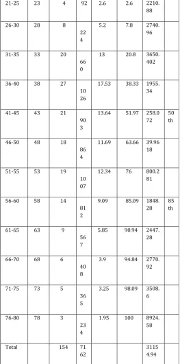
Speed percentiles are tools used to determine effective and adequate speed limits. The two speed percentiles most important to understand are the 50th and the 85th percentiles. The 50th percentile is the median speed of the observed data set. This percentile represents the speed at which half of the observed vehicles are below and half of the observed vehicles are above. The 50th percentile of speed represents the average speed of the traffic stream. The 85th percentile is the speed at which 85% of the observed vehicles are traveling at or below. This percentile is used in evaluating recommending posted speed limits based on the assumption that 85% of the drivers are traveling at a speed they perceive to be safe (Homburger et al. 1996). In other words, the 85th percentile of speed is normally assumed to be the highest safe speed for a roadway section. Weather conditions may affect speed percentiles. For example, observed speeds may be slower in rainy or snowy conditions. A frequency distribution table is a convenient way to determine speed percentiles. An example is given in “Table 2,” The frequency of vehicles is the number of vehicles recorded at each speed.

Σ fi(vi − vm)2 = 31154.94 (1)

Σ fi −1 = 154-1 = 153 (2)

The cumulative frequency is the total of each of the numbers (frequencies) added together row by row from lower to higher speed. The fourth column is a running percentage of the cumulative frequency.

The 50th and 85th speed percentiles are determined from the cumulative percent column. For example data in “Table 2,” the 50th_{percentile falls between 41 and 45 kmph and the} 85th percentile falls between 56 and 60 kmph.

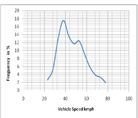
The calculation of speed percentiles is easier if a sample size of 100 vehicles is collected. When the sample size equals 100 vehicles, the cumulative frequency and cumulative percent are the same. The analysis of an example set of speed data is shown in “Table 3”. The data are first grouped into intervals of 5 km/h. The first two columns of the table show the grouping by lower limit, midpoint of mean (VI), and upper limit of each group. Column 3 shows the frequency (fi) or

number observed in each group; column 5 shows the

percentage of observation in class.

(4)

The arithmetic average or mean speed is the most frequently used speed statistic. It is a measure of the central tendency of the data and is computed from the formula:

𝑣 = Σ 𝑓𝑖𝑣𝑖 = 46.51

Σ 𝑓𝑖

Where: 𝑣 = mean or average speed.

Σfi Vi = sum of the mean frequencies

Σf I = total number of vehicles observed (total of Col.3)

s. n o Type of vehicl e

5 1 0 1 5 2 0 2 5 3 0 3 5 4 0 4 5 5 0 5 5 6 0

1 Car and taxi 2 0 2 5 1 8 2 3 8 6 2 Small van and utility 1 8 2 1 1 7 2 3 7 9

3 Moder ate size lorry and large van 1 2 1 6 1 7 1 9 6 4 4 Truck 1 2 1 0 1 3

9 4 4

5 Bus

5 2 6 4 1

[image:4.595.34.561.66.802.2]

7 6 Motor cycle 1 0 5 1 0 9 1 0 1 1 1 2 4 2 7 Total( veh/h) 1 7 2 1 8 3 1 7 2 1 9 9 7 2 6

[image:4.595.317.553.70.352.2]

Table 1 VEHICLE TALLLY SHEET

Figure 5 vehicle volume data count

SAMPLE MEASUREMENT SHEET FOR SPOT SPEED DATA COLLECTION DATE: 6 June 2017

TIME: 10:30 A.M. LENGTH: 50 METER

METHOD USED: PAVEMENT MARKING

TABLE 2 S.N O Car/jee p Three wheele r Two Wheele r cycl e H.C.V. (HEAVY COMMERCI AL VEHICLE) L.C.V. (LIGHT COMMERCI AL VEHICLE)

1 2.94 3.49 2.87 5 5.8 3.45

2 2.51 3.9 2.89 8.2 5.4 3.46

3 4 4.8 2.94 6.9 3.48 3.45

4 2.5 3.48 2.9 8.2 3.22 2.91

5 2.85 4.31 3.43 6.89 5.9 3.2

6 4 3.9 2.68 8.2 3.48 3.21

7 2.49 3.49 3.10 6.9 6.9 3.45

8 2.4 4.31 3.43 5.8 3.48 3.9

9 3.22 4.31 3.10 6.9 3.21 3.45

(5)

12 5 4.5 3.15 8.23 5.9 3.9

13 2.3 3.9 3.43 8.24 6.9 3.25

14 5 4.33 2.87 8.25 6.92 3.84

15 2.7 4.5 3.91 8.32 3.98 4.6

16 2.54 3.9 3.43 8.23 4.01 4.7

17 2.68 4.33 3.15 8.1 4.23 3.85

18 2.32 4.5 4.3 8.12 4.5 4.65

19 2.36 4.5

20 2.68

[image:5.595.35.293.100.570.2]

21 3.95

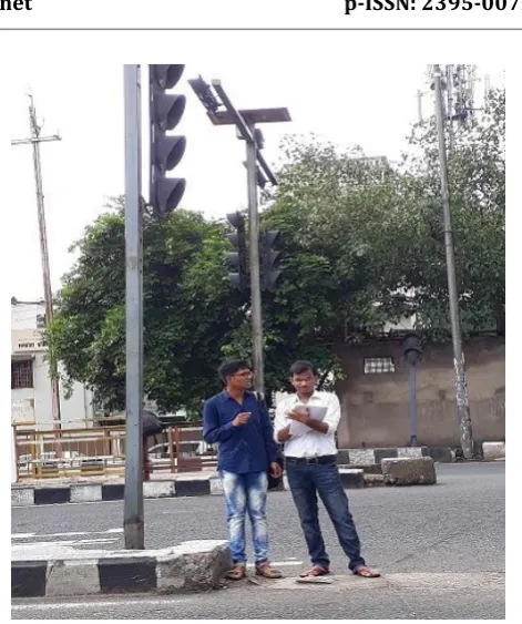
Fig 6 marking of start point for spot speed data Collection

C .Distributions in Time and in Space

Data collected at a point over a period of time, e.g.: by stopwatch or radar meter, produce speed distributions in time, whose means are time mean speeds. Data obtained over a stretch of road almost instantaneously as by two successive aerial photographs, result in speed distribution in space and space mean speeds.

These distributions are not the same; time mean speed is higher than space mean speed. This can be understood if one visualizes a section of highway; a spot speed sample at one end taken over a finite period of time will tend to include some fast vehicles which had not yet entered the section at

[image:5.595.308.580.140.442.2]

the start of the survey, but will exclude some of the slower vehicles which were within the highway section when the sample was started.

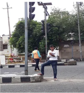
Figure 7 spot speed data collection on measurement sheet

An aerial photograph, however, would include all vehicles within the highway section at the moment of exposure. The relationship between the two mean speeds is expressed by:

𝑉 𝑡 = 𝑉𝑠 + = 46.51+14.269 = 60.779

where Vt and Vs are the time mean speed and space mean speed respectively, and ss_{is the standard deviation of the}

distribution in space.

Speed

class(km /hr)

Class

midva lue vi

Class frequen cy

(numbe r of

observa tions in

class)

Fi

Fi *

vi

Percent age of

observa tion in class

Cumula tive

percent age of all

observa tion

(6)

88

26-30 28 8 22 4

5.2 7.8 2740. 96

31-35 33 20 66 0

13 20.8 3650. 402

36-40 38 27 10 26

17.53 38.33 1955. 34

41-45 43 21 90 3

13.64 51.97 258.0 72

50 th

46-50 48 18 86 4

11.69 63.66 39.96 18

51-55 53 19 10 07

12.34 76 800.2 81

56-60 58 14 81 2

9.09 85.09 1848. 28

85 th

61-65 63 9 56 7

5.85 90.94 2447. 28

66-70 68 6 40 8

3.9 94.84 2770. 92

71-75 73 5 36 5

3.25 98.09 3508. 6

76-80 78 3 23 4

1.95 100 8924. 58

Total 154 71 62

[image:6.595.30.294.100.633.2]

3115 4.94

TABLE 3 PERCENTAGES AND ANALYSIS OF SPOT SPEED DATA

All vehicles do not travel at the same speed, so there is a spread or dispersion of speeds about the mean. The standard deviation, s, is a statistical measure of this spread.

Assuming a normal distribution, the mean I plus and minus one standard deviation contains approximately 68% of the vehicles, plus and minus two standard deviations contains

95%, and plus and minus three standard deviations contains 99.8%. The standard deviation of the sample is computed by first calculating the variance of the sample and then taking the square root as follows:

S = =14.269 km/h

Where: S = standard deviation of the distribution Σ fi(vi − v) = sum of the mean square frequencies

Σ fi(vi − v)^2 = square of the sum of the mean frequencies

(total of Col. 7 squared )

D. Standard Error of the Mean

The means of different samples taken from the same population are distributed normally about the true mean of the population with standard deviation of S/ where a is the standard deviation of the entire population. In large samples (n ≥ >25) the standard deviation of the sample, s, is a good estimate of the standard deviation of the population. Therefore:

𝑠𝑣 2 =

𝑠𝑣 = =14.269/154= 1.322

Where 𝑠𝑣 2 = variance of the mean

𝑠𝑣 = standard error of the mean

𝑠2 = sample variance (from equation)

V. GRAPHICAL ANALYSIS

The cumulative percentage calculated in “Table 3” is plotted against the upper limit of each speed group. A smooth S-shaped curve drawn approximately through the points (not connecting the points directly) is called the cumulative speed curve. Since the sample is used to estimate the total distribution, it is important that it be a smooth curve rather than a joining of points.

The data in “Table 3” are plotted and the corresponding cumulative speed curve is drawn in Fig 8. Significant values obtained from the curve shown on the figure are:

The vertical axis of the curve is the percentage of vehicles traveling at or below the indicated speed. Any specific percentile speed is the speed that corresponds to the desired percentile. The uses of some of the percentiles are as follows:

(1) The Median (50th Percentile) Speed is an alternative

(7)

equals the mean value. The median is obtained from the curve by reading the speed that corresponds to the 50% value.

(2) The 85th Percentile Speed, sometimes referred to as

the critical speed, is used as a a guide in establishing reasonable speed limits.

(3) The 15th Percentile may serve as the guide for

[image:7.595.260.561.64.526.2]

establishing minimum speed limits. The vehicles traveling below this value tend to obstruct the flow of traffic, thereby increasing the accident hazard.

TABLE 4

PCU VALUES

PCU/HR PERCENTAGE OF PCU

1 86 8.90 2 158 16.37 2.5 160 16.56 3 132 13.67 3 51 5.28 1 427 44.203

966 100

Figure 8 Cumulative Distribution

VI. CONCLUSION AND RECOMMENDATION

[image:7.595.308.570.91.314.2]

Unlike many other disciplines of the engineering, the situations that are interesting to a traffic engineer cannot be reproduced in a laboratory. Even if road and vehicles could be set up in large laboratories, it is impossible to simulate the behavior of drivers in the laboratory.

Figure 9. Frequency Distribution

0 10 20 30

21

-25

26

-30

31

-35

36

-40

41

-45

46

-50

51

-55

56

-60

61

-65

66

-70

71

-75

76

-80

O

b

se

rv

e

d

fr

e

q

u

e

n

cy

Vehicles speed (km/h)

[image:7.595.36.292.259.614.2]

Histogram of observed

vehicles

Figure 10. Histogram of Vehicles Speed

Therefore, traffic stream characteristics need to be collected only from the field.

The data was collected on the Hoshangabad road - National Highway – 12 and was analyzed with the Following results: The data was collected on the Hoshangabad road - National Highway -12 and was analyzed with the Following results:

1. The maximum speed on the road is equal to 80. The drivers almost do not exceed this speed. It was corroborated by our analysis where the vehicles were moved with the range of speed from 30 to 70 km/h.

2. The most part of vehicles moved with average speed 45 km/h.

[image:7.595.320.559.354.510.2]

(8)

(427 vph).

5. Some of the results can have natural error that is result of purposefully decreasing of speed. Because observation group can be easily detected by drivers from the long distance.

6. This particular area does contain a signboards about speed limit of 30km/hr and some of the drivers over exceed the speed limit (km/h).so it should be ensured that drivers don’t breakup speed limit

VII.REFERENCES

[1] Khanna, S.K., And Justo, C.E.G., (1993), “Highway Engineering”, New Chand And Bros, 7th Edition, New Delhi.

[2] Nicholas J. Garber, Lester A. Hoel ,(2009) , “ Traffic and

Highway engineering “ , 5th edition , U.S.A.

[3] ITE, Brian Wolshon, Anurag Pande (2016) , “ Traffic

engineering handbook “ , 7th edition , New Jersey.

[4] Thomas R. Currin (2012) , “ Introduction to traffic

engineering’’, 2nd edition . U.S.A

[5] Dr. L.R. Kadiyali , “ Traffic Engineering and transport planning ” , 9th edition , New Delhi.

[6] F D Hobbs. ,(1979), ‘’ Traffic planning and engineering ”, 2nd edition.

[7] Theodore M Matson , Wilbure S smith , fedric W Hurd , (1955)

Evaluation of Traffic Characteristics: a Case Study on NH 12, Near Barkatullah University, Bhopal (M P )