A Novel Method to Identify the Global Sources and Sinks of Carbon Dioxide Based on Spatial Analysis

http://dx.doi.org/10.4236/jgis.2015.72010

A Novel Method to Identify the Global

Sources and Sinks of Carbon Dioxide Based

on Spatial Analysis

Ali Madad

, Babak Naimi

, Saeidi Anjileh Mehdi

1_{Department of Environment and Energy, Faculty of Science and Research Branch of Islamic Azad University,}

Tehran, Iran

2_{Department of GIS/SDI, National Cartography Center of Iran, Tehran, Iran}

Email: *_{[email protected]}

Received 12 March 2015; accepted 3 April 2015; published 7 April 2015

Copyright © 2015 by authors and Scientific Research Publishing Inc.

This work is licensed under the Creative Commons Attribution International License (CC BY). http://creativecommons.org/licenses/by/4.0/

Abstract

Today global warming has become one of the most important concerns of environmental science. The redundancy of greenhouse gases in the atmosphere is known as a major factor in this pheno-menon. These gases contain water vapor, carbon dioxide, methane, nitrous oxide, and ozone. The CO2 gas is one of their most effective among these gases. According to scientific warnings, the amount of CO2 gases in the atmosphere has increased by 40% to 45% over the last 50 years. Re-ducing the abundant gas in the atmosphere requires a good knowledge of related factors involved, including sources that emit gases into the atmosphere and sinks that absorb the gas from the at-mosphere. The amount of CO2 gas in the atmosphere has been accurately measured in previous years with great certainty. But the predicted values of emissions from sources and removals by sinks have large ambiguities. As studies show, even the computed residuals trends (which is ob-tained by subtracting the amounts of sinks from sources) strongly disagree with the trends of the existence of CO2 in the atmosphere. This study as a preliminary review, proposes a method to identify the locations of sources and sinks of carbon dioxide using global statistical information and adding spatial analysis approaches. By applying this method to the data observed from 2000 to 2011 and the extraction of likely sources and sinks, the region of the Black Sea, near Romania recognized as one of the strong points issued and Bukit Kototabang near Indonesia acknowledged as an Impressive CO2 absorption zone.

Keywords

Carbon Dioxide Sink, Spatial Autocorrelation, Interpolation, Volcanic Shape

changes in temperature and precipitation in Tabriz city in terms of doubling of atmospheric carbon dioxide con-clude that in this case, the temperature for all seasons increase significantly [3]. Carbon dioxide measurements in the atmosphere are very precise and show the annual growth of the accumulation in the atmosphere of the earth. Despite this certainty, the amount of carbon dioxide produced by the earth cannot be determined yet. Also the amount of gas absorbed by the land and oceans is not determined [4], although a substantial sum is formed. For example, the most important way of reducing carbon dioxide in the atmosphere after reducing the consump-tion of fossil fuels is carbon storage in terrestrial ecosystems and land. Soil contains 75% of the land carbon source [5]. Determining the emission or absorption of carbon dioxide in the atmosphere requires a detailed knowledge of at least one of them. By subtracting the amount of gas in atmosphere we can obtain the other. Reaching this trust requires a wide range of global geophysical and economic data. Corinne Le Quéré (2009) prepared an overall rate of all production and absorption of carbon dioxide from 1959 to 2008 to develop and analyze the phenomena that affect them. The growth rate of carbon dioxide in the atmosphere was determined on the basis of direct measurements. The amount of carbon dioxide produced by fossil fuels was detected ac-cording to statistics from the consumption of fossil fuels in different countries. The amount of carbon dioxide that comes from land use changes was estimated by statistical deforestation, land use, spatial observations fires, and assumptions about the carbon density in the vegetation and soil. The result of the operation shows that the amounts of the estimated residuals were not compatible with the quantity of gas in the atmosphere. The inability to identify the source and extent of absorption and excretion of carbon dioxide prevents accurate understanding of the carbon cycle [4]. The purpose of this article is to present a method to identify locations where gas adsorp-tion or desorpadsorp-tion may have occurred. This method works by implementing spatial analysis in the global statis-tical information quantities of gas in the atmosphere.

2. Source and Sink Trends

Most studies on the precise knowledge of the factors that influence the uptake and release of carbon dioxide be-gan around the 1990s. These studies can be divided into two groups: 1) Assessment of changes in carbon dio-xide in the atmosphere, and understanding the effective factors that cause them. 2) Statistical analysis of climate data and maps to predict the spread and absorption of gases. If the amount of carbon dioxide in the atmosphere is the balancing result of known sources and sinks, according to the known factors that influence the absorption and release of carbon dioxide gas the budget can be shown as indicated by the following equation [6]:

Fossil+Land Use+Ocean+Terrestrial Biota=Trend (1)

The trend of carbon dioxide in the atmosphere is equivalent to the sum of the amount of gas emitted by the sources and absorbed by the sinks. According to measuring stations on the surface of the Earth, an average of 40% of the total annual CO2 emissions between 1959 and 2008, remain in the atmosphere. But this number, as shown inFigure 1 [4] [7], has also high annual variations too.

The amount of CO2 emission values with the absorbed CO2 is called residual values. The trend chart is shown inFigure 2 [4] [8]. The range in which the shadow appears, the calculation is approximate.

As the comparison betweenFigure 1 andFigure 2 shows, the trend of changes in atmospheric carbon dioxide does not justify the fluctuations of its calculated residual amounts. In other words, the growth rate of CO2 in the atmosphere does not correspond with the calculated emissions and absorptions [4].

Figure 1. The annual fluctuations of CO2 emissions in the

atmosphere [4] [7].

Figure 2. Residual annual fluctuations in atmospheric CO2

[4] [8].

3. Material and Methods

All arithmetic operations used in the studies mentioned in the previous section, are often limited to the statistical analysis of (non-spatial) descriptive data, while the spatial resolution with its good analytical equipment that is able to identify areas with certain characteristics in the environment is suitable to apply. The importance of the method presented in this study is its approach in using this kind of analysis.

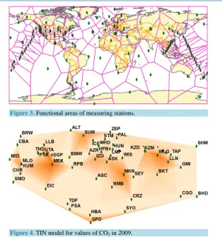
The data used in this study were carbon dioxide values in the atmosphere between 2000 and 2011 that is measured by 63 sampling stations, through the database offered in GLOBAL VIEW. Information available on this site starts from 1999. Prior to 1988, the number of measurement stations was much less. Studies show that at least 10 stations for each study area are required to obtain good estimates [9]. The samples are offered both daily and monthly. By calculating the average of monthly data, annual values for each station were calculated and used. Using the geographical coordinates of stations and a view of world map, the working platform was prepared. Using polygon analysis of Thiessen, the functional areas of each station is shown inFigure 3.

Using annual data for each station and their geographical positions, a Triangular Irregular Network (TIN) model was produced.Figure 4 illustrates an example of this model for 2009.

Then by using the TIN models, the contour maps were generated from them. By implementing a method that will be explained in the next section, for each station a numerical value proportional to its role in the sink or source of the region obtained. These values are named in this paper by “Stations Volcanic Degree” (SVD). In conclusion, the amounts of these SVDs were compared during 2000-2011.

3.1. Stations Volcanic Degree (SVD)

The objective is that with the help of obtained models, the areas where they can absorb or emit gases are identi-fied. TIN models are something like the earth terrain. It is possible to see some lumps and troughs over them. Height of the hills or mountains illustrates the high amount of value in that area. And depth of the valleys shows the low amount of the value over there.

Figure 3. Functional areas of measuring stations.

Figure 4. TIN model for values of CO2 in 2009.

feature leads to the concept of detecting volcanic forms in the TIN models to find the places where the emission or absorption was occurred. The volcanic mountains have their own characteristic shapes. InFigure 5, the three main types of volcanic formation are reported [10]. In this view, the formations of peaks are more important than their heights. For example, the elevated Himalayan peaks over 8000 meters are considered much more non-volcanic mountains than a single volcanic mount such as Ararat or Damavand with their less than 6000 me-ters height.

Because of the symmetry, the same calculation for the identification and classification of volcanic peaks was used to identify canyons in the reverse mode (gas resources or reductions).

Similar to the individual characteristics of volcanic peaks, with the method shown in Figure 6, and using contour maps, the characteristics of peaks and valleys were extracted and initialized their SVDs values based on the amounts of volumes enclosed by them. It is assumed that the absolute value of SVD indicates the possibility of locating the gas creative factor in the position of the station.

3.2. Model Validities

This research was conducted in two types of validations: 1) The existence of a spatial relationship between the numerical values of measurement stations. 2) Evaluation of Triangular Irregular Network model (TIN). The fol-lowing sections explain how to perform each of these surveys.

3.2.1. Validating Spatial Relationship

Figure 5. Three main types of volcanoes [7].

omitting not closed poly lines

The rings sorted from smallest to the largest, and the station which locates inside

the first ring is chosen as the first peak

Does there exist an old peak inside the ring?

The ring belongs to the old peak The ring belongs

to the new peak

Omitting peaks which contain less than 3 rings

once again examining the rings and omitting those which the number of peaks in their

interior are different from 1

Yes No

defining the closed volume between the peak and its outer ring as the related Station Volcanic Degree (SVD)

Figure 6. The SVDs rankings for assessing stations.

i j

∑ ∑

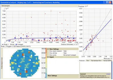
n is the number of samples in the specified interval. Consequently, the calculation leads to a graph which shows the amount and type of the spatial relationship between the values.Figure 7 shows the result of this operation for the values of stations in 2009.

The charts show the existence of spatial relationship of exponential type, between the values of stations in 2009. Therefore, the spatial analysis on the data is acceptable

3.2.2. Validating TIN Model

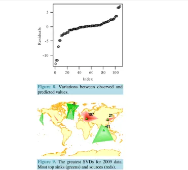
TIN models are generated by interpolation processes. For validating the interpolation method, 15% of the sta-tions was kept and with the rest of them a three dimensional surface was generated by TIN Model. Then the predicted values of TIN model for the locations of the excluded stations were compared to their actual values. The test was performed 20 times with the 2009 data. Average relative error of 0.7% was achieved in the experi-ments. So, the use of the TIN model for the spatial analysis of stations values is acceptable.Figure 8 shows the relative errors that have been drawn in ascending order.

As it is shown, the main results of errors are around zero. There are some cases that have much difference. These cases may be a sign of the gas emission or absorption in their areas.

4. Results

Figure 9shows an example of the results of this paper in relation to 2009 data.

Figure 8. Variations between observed and predicted values.

Figure 9. The greatest SVDs for 2009 data. Most top sinks (greens) and sources (reds).

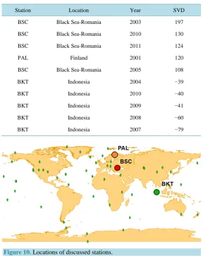
In this case, the strongest peak, with 107 SVD value is known at the BSC station in the “Black Sea” area. The strongest valley with SVD value of −41 is known at the BKT position near “Indonesia”. With these assumptions, the probability that in 2009 at the Black Sea region a strong CO2 emission factor being founded is much more than any other place. In addition, the gas absorption factor in the position of Indonesia station will be more dis-coverable. By applying the proposed method, to CO2 values of stations during 2000 to 2011, the 12 maps were produced. In each map the peaks and valleys were illustrated. The peaks and valleys were graded with their SVD values.Table 1 shows 10 stations that have the highest degree of positive and negative values of SVD.

Table 1show that there is a strong domination in the BSC and BKT stations from all others. The station of the Black Sea (BSC), with its high SVD values, shows the highest degree of CO2 emission zone, and can be a good option for discovering the CO2 emission factors. This inference exists while the average values measured at the station is something close to the average of the others, and apparently no particular dominance over others, can be seen. And the Indonesia station (BKT) is recommended as a priority area for detecting CO2 gas absorp-tion factors. The SVD value of the PAL staabsorp-tion has always been negative, and only in 2001 became largely posi-tive. It can also be a sign of a temporary source of CO2 emissions in 2001 in the region.Figure 10shows the location of these stations.

5. Conclusion

PAL Finland 2001 120

BSC Black Sea-Romania 2005 108

BKT Indonesia 2004 − 39

BKT Indonesia 2010 − 40

BKT Indonesia 2009 − 41

BKT Indonesia 2008 − 60

BKT Indonesia 2007 −79

Figure 10. Locations of discussed stations.

mentioned in the previous sections, despite the extraordinary importance of preventing the growth of residual carbon dioxide in the atmosphere, the identification of factors that influence the emission and absorption of the gas is extremely low and rough. The method proposed in this paper is an innovative approach compared to pre-vious studies, and expresses the results quickly and explicitly. It is good to use a method to evaluate the results of this study with cases of observation. In addition, because the residual quantity of atmospheric carbon dioxide is strongly dependent on the temperature, it is good to do this research, again with seasonal data, and the results reviewed.

Acknowledgements

I would like to deeply thank Dr. Ali Javidaneh who cooperated in the development of research ideas. And also Mr. Nima Ghasemloo and Dr. Hamid reza Ranjbar who helped me frankly in implementing the computer pro-grams for this study.

References

[1] Atherton, J. (2012) Multiscale Remote Sensing of Plant Physiology and Carbon Uptake. Thesis for the Degree of

Doc-tor of Philosophy to the University of Edinburgh, Edinburgh.

[2] Azizi, G. and Karimi, M. (2005) Thermal Trend in Passed 10 Years in Iran. Geographical Science Journal, 4, 22-29.

[3] Salahi, B. and Valizadeh, Kh. (2006) Thermal and Precipitation Changes Simulation in Tabriz by Doubling the

[4] Le Quéré, C., Raupach, M.R., Canadell, J.G., Marland, G., et al. (2009) Trends in the Sources and Sinks of Carbon

Dioxide. Nature Geosciences, 2, 831-836. http://dx.doi.org/10.1038/ngeo689

[5] Tan, R.R. (2010) Determining Approximate Stackelberg Strategies in Carbon Constrained Energy Planning Using a

Hybrid Fuzzy Optimisation and Adaptive Multi-Particle Simulated Annealing Technique. The Institution of Engineers, Malaysia, September 2010, 71-3

[6] Badeban, Z. and Zahedi, Gh. (2008) Considering the Carbon Sequestration in Forest Soil. Forest and Timber

Produc-tion Journal, 62.

[7] Canadell, J.G., et al. (2007) Contributions to Accelerating Atmospheric CO2 Growth from Economic Activity, Carbon

Intensity, and Efficiency of Natural Sinks. Proceedings of the National Academy of Sciences of the United States of

America, 104, 18866-18870. http://dx.doi.org/10.1073/pnas.0702737104

[8] Denman, K.L., et al. (2007) Couplings between Changes in the Climate System and Biogeochemistry. In: Solomon, S.,

et al., Eds., IPCC Climate Change 2007: The Physical Science Basis, 499-587, Cambridge University Press, Cam-bridge.

[9] Fan, S., Gloor, M., Mahlman, J., Pacala, S., Sarmiento, J., Takahashi, T. and Tans, P. (1998) A Large Terrestrial

Car-bon Sink in North America Implied by Atmospheric and Oceanic CarCar-bon Dioxide Data and Models. Science, 282,

442-446. http://dx.doi.org/10.1126/science.282.5388.442

[10] Manconi, A., Walter, T.R. and Amelung, F. (2007) Effects of Mechanical Layering on Volcano Deformation.