© 2017, IRJET | Impact Factor value: 5.181 | ISO 9001:2008 Certified Journal
| Page 1677
Comprehensive Approach towards Modelling and Simulation of
Single Area Power Generation System Using PI Control and
Stability Solution Using Linear Quadratic Regulator
,
1
Graduate Student, Dept. of Electrical Engineering, Rochester Institute of Technology, Dubai, UAE
2
Professor, Dept. of Electrical Engineering, Rochester Institute of Technology, Dubai, UAE
---***---Abstract -
In this paper, the open loop single area powergeneration system is modelled using state space representation. The output response which is frequency deviation at steady state is simulated using MATLAB. Then, Proportional Integral (PI) controller is added to the system to understand the effect of a conventional controller on system steady state output response. The controlled system is stabilized through design of Linear Quadratic Regulator (LQR). The performance of system steady state output response is measured in terms of undershoot percentage, settling time, and steady state error. The controlled system simulation at the end of this paper shows that PI control is an efficient, reliable, and robust technique to solve power generation system optimization problem. The output response of the considered controlled system has settling time of 0.7 second, zero steady state error, and undershoot of 5.45%.
Key Words:
Optimization, Single Area Power
Generation System, LQR Technique, PI Controller, Steady State Response1
INTRODUCTION
An interconnected system called Automatic Generation Control (AGC) consists of two sub-systems: Load Frequency Control (LFC) and Automatic Voltage Regulator (AVR). AVR is responsible to regulate the terminal voltage and LFC is employed to control the system frequency. In this paper, modelling and simulation of LFC is considered for careful analysis since LFC is more sensitive to changes in load compared to AVR. LFC and AVR are decoupled and can be analyzed separately. There is only weak overlap of effect between the two sub-systems [1].
Optimizing thermal power generation system will reduce energy or fuel consumption. Fuel reduction of even a small percentage will lead to large energy saving which results into saving the environment [2]. Hence, many researchers have been interested to solve optimization problem in thermal power generation systems. In order to optimize power generation system, the plant has to operate at
desired operating level which corresponds to operating at nominal frequency.
2
OPEN LOOP ANALYSIS
Figure 1 shows the SIMULINK generated block diagram of an uncontrolled generating unit which consists of a speed governor, a turbine, a re-heat, and a generator [1]. The inputs of the system are Δ representing the change in speed generation by utility and Δ representing the change in load by consumer also known as disturbance. Since user has no control over load changes, Δ is
considered the only input of the system. The effect of Δ will be disappeared when a controller is added to the system.
The fact that the frequency changes with load generation imbalance gives an accurate way to regulate the imbalance. Hence, frequency deviation Δf is considered as a regulation signal to study the system performance. The output of LFC is Δf which represents the change or variation in steady state frequency. The objective is to have a constant output frequency which corresponds to Δf being zero or very small. The value of Speed Regulation R also known as Droop is the ratio of frequency deviation (Δf) to change in power output of the generator. Table 1 shows the constants used for single area power system in Figure 1.
Table -1: List of Constants
Symbol Description Value
Governor Time Constant 0.4sec
Turbine Time Constant 0.5sec
Re-heat Time Constant 10sec
Generator Time Constant 20sec
Re-heat Gain Coefficient 0.5
Generator Gain Coefficient 125
© 2017, IRJET | Impact Factor value: 5.181 | ISO 9001:2008 Certified Journal
| Page 1678
Fig -1: Block Diagram Representation of Single Area Power Generating UnitThe output of each integrator in Figure 1 is a state variable. Hence, state variable matrix A must be a 4x4 matrix. Equations 1-4 show the developed transfer functions:
Generator
= (1)
Re-heat = (2)
Turbine = (3)
Governor = (4)
To develop state space representation of the system shown in Figure 1, rate of change of each state variable is needed. Therefore, Inverse Laplace Transform of the transfer functions shown in Equations 1-4 is taken and the equations are re-arranged into equations 5-8: ̇ = + - Δ (5)
̇ = + + (6)
̇ = + (7)
̇ = - (8)
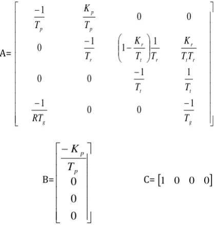
Then, Equations 5-8 are transformed into state space model. It is important to note that the output of the system Δ is the state variable . Hence, the output matrix C will be a row matrix of size 1x4. The input matrix B is a matrix of size 4x1. State Space representation of any system follows the following structure: ̇ =A x(t) + B Δ (9)
y(t)= C x(t) (10)
Following is state space representation of LFC shown in Figure 1:
A=
g g
t t
r t
r
r t r
r p p
p
T RT
T T
T T
K T T K T
T K T
1 0
0 1
1 1
0 0
1 1 1 0
0 0
1
B=
0
0
0
p pT
K
[image:2.595.309.521.234.454.2]C=
1 0 0 0
Figure 2 illustrates the output response of the LFC model generated in MATLAB. The input Δ is a unit step function. The output response begins with oscillations and dampens at steady state. Since there is increase in load, undershoot is expected. Increase in load leads to decrease in frequency which corresponds to undershoot. Decrease in load leads to increase in frequency which corresponds to overshoot. The settling time of the system is 150 seconds and the steady state value is -2.5 HZ. The undershoot percentage, settling time, and the steady state value are significantly large and this leads to the necessity of having a controller added to the system.
[image:2.595.88.285.453.531.2] [image:2.595.309.557.618.747.2]© 2017, IRJET | Impact Factor value: 5.181 | ISO 9001:2008 Certified Journal
| Page 1679
3
CONVETIONAL CONTROLLERS
The primary objective of having a controller in power system is to eliminate the steady state frequency deviation. In any reliable power system, following specifications are expected to be met:
1. Steady state frequency error should not be more than 0.01HZ.
2. Settling time should be less than 1 second. 3. The maximum undershoot should not be more
than 6% which corresponds to transient frequency of 0.06HZ.
Each controller has different role. Proportional controller is used to reduce rise time and settling time. Integral controller is used to eliminate steady state error. The negative effect of integral controller is creating oscillation. Derivative controller is used to improve transient response which means reducing overshoot/undershoot. Equations 11-15 show structure of most commonly used conventional controllers where U(s) is the controller output and E(s) is the controller input.
Proportional (P): U(s) = E(s) (11)
Integral (I): U(s) = E(s) (12)
Derivative (D): U(s) = S) E(s) (13)
PI: U(s) = E(s) (14)
PID: U(s) = E(s) (15)
Area Control Error (ACE) is the difference between actual power flow out of area and scheduled power flow. Ideally, the main objective in optimization problem is to improve the dynamic response of the system by minimizing or even eliminating AEC. In other words, the main objective is to lead each utility to constantly change its generation to follow the ACE. In real life power systems, it is rare to have no ACE due to instantaneous change in load. Hence, the objective is to keep AEC as close to zero as possible. Integral control is well suited in this purpose.
4
FEEDBACK ANALYSIS
For single area closed loop system, a Proportional Integral (PI) controller is added to the system as shown in Figure 3. Equation 14 shows the transfer function of the PI controller used in this section. The system shown in Figure 3 has 5 integral blocks which corresponds to 5 state variables. Equations 16-20 show the transfer functions of each integral block in Figure 3 where is the proportional constant and is the integral constant. Generator = (16)Re-Heat = (17)
Turbine = (18)
Governor = (19)
PI Control = (20)
Inverse Laplace Transform of Equations 16-20 are taken and the equations are re-arranged into differential Equations 21-25 to find rate of change of each state variable. ̇ = + - Δ (21)
̇ = + + (22)
̇ = + (23)
̇ = - - (24)
̇ = ( + - Δ (25)
Fig- 3: Block Diagram Representation of Feedback Single Area Power Generating Unit
© 2017, IRJET | Impact Factor value: 5.181 | ISO 9001:2008 Certified Journal
| Page 1680
=
0
0
0
1
1
0
0
1
0
1
1
0
0
0
)
1
(
1
1
0
0
0
0
1
\ p p g p g i g g g t t t r r t r r r p p pT
K
K
T
K
K
T
T
RT
T
T
T
T
K
T
K
T
T
T
K
T
=
p p g p pT
K
K
T
K
0
0
0
=
1
0
0
0
0
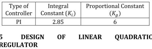
[image:4.595.31.265.71.385.2]PI tuning is a challenging task as the parameters of the controller need to be changed until the desired requirements are met. Table 2 shows the nominal values of the PI controller used in Figure 3.
Table 2: Controller Parameters for Feedback Single Area Generating Unit
Type of
Controller Constant (Integral Proportional Constant
PI 2.85 6
5
DESIGN
OF
LINEAR
QUADRATIC
REGULATOR
When a controller is added to a system, a new pole is in fact added to the system which may cause the system to become unstable. This means a stabilizing technique is essential. When a system is controllable, optimization will automatically stabilize the system. However, if the system is uncontrollable, optimization will not stabilize it. Therefore, it is crucially important to check controllability of the system before optimizing it.
To check controllability of the system, rank of controllability matrix must be checked using Equation 26.
=
B
AB
A
2B
A
3B
A
4B
(26)Rank of the matrix shown in Equation 26 is 5 which is equal to the size of the system. Hence, the system is controllable and Linear Quadratic Regulator (LQR) technique guarantees stability.
In optimization using LQR method, The Error Weighted MatrixQ(t) and The Control Weighted MatrixR(t) need to be selected wisely such that the system given specifications are satisfied. Q(t) and R(t) are symmetric matrices. The simplest way to choose Q(t) matrix is to start with an identity matrix. The size of the identity matrix depends on the number of state variables used in the system modelling. Power system is an output regulator system since the objective is to keep the output Δf close to zero. Hence, in Q(t) matrix the most important element is the element that is directly related to the output. The R(t) matrix is related to input of the system. A system with n inputs requires R(t) matrix of size nxn. Increasing value of R will increase the implementation cost. Hence, it is important to choose a small value for R(t). Once Q(t) and R(t) matrices are selected, MATLAB can design the controller. Q(t)=
1
0
0
0
0
0
1
0
0
0
0
0
1
0
0
0
0
0
1
0
0
0
0
0
8
.
14
R(t)=
0.2Matrix K is the feedback gain matrix generated by Matlab.
K=
2
.
565
0
.
305
0
.
431
1
.
125
2
.
322
The optimal control law shown in Equation 27 will generate a new state matrix as shown in Equation 26 [3].
U= - K X(t) (27)
= - K (28)
generates a feedback stable system with the
following eigenvalues: -99.5547 + 0.0000i, -2.7414 + 0.6461i, -2.7414 - 0.6461i, -2.6055 + 0.0000i, -0.1183 + 0.0000i.Since all the five poles are located on the left-half plane, the closed loop system is a stable system.
6
RESULTS
Figure 4 is MATLAB generated output response of the optimized system modelled in Figure 3. Based on the simulation result, the system is stable and the steady state
[image:4.595.38.286.480.560.2]© 2017, IRJET | Impact Factor value: 5.181 | ISO 9001:2008 Certified Journal
| Page 1681
shown in Figure 5.Fig-5: Comparison of Controlled vs Uncontrolled Output Response
7
CONCLUSION
type of conventional controller is suitable for a specific purpose. Based on the specifications given for power generation system, a PI controller has been selected. The parameters of the controller which are integral gain and proportional gain have been tuned in MATLAB till the desired response is achieved. LQR method was used to stabilize the controlled system. Response of the controlled system had settling time of 0.7second, undershoot of 5.45%, and zero steady state error.
REFERENCES
[1] Dr. A. Ismail, Professor of Electrical Engineering at Rochester Institute of Technology, Dubai, UAE. Advances in Power Generation System (2017). [2] P. Pechtl. Integrated Thermal Power and
Desalination Plant Optimization. PowerGen Middle East, Paper No.110 (2003).
[3] R. Boruah, Dr. B. Kanta Talukdar. Modelling of Load Frequency Control Using PI Controller and Stability Determination with Linear Quadratic Regulator. Assam Engineering College. India (2014)
.
BIOGRAPHIES
Nastaran Naghshineh is a
graduate of Electronics
Engineering from Simon Fraser University, British Columbia, Canada. Currently, she is completing her Master’s degree in Electrical Engineering, specializing in Control System, at
Rochester Institute of
Technology (RIT) Dubai, UAE. Email: [email protected]
Dr. Abdulla Ismail obtained his B.Ss (’80), M.Sc. (’83), and Ph.D. (’86) degrees, in Electrical Engineering from the University of Arizona, U.S.A. Currently, he is a full professor of Electrical Engineering and assistant to the President at Rochester Institute of Technology (RIT) Dubai, UAE. Email: [email protected]
Fig-4: Feedback System Output Response
For easier comparison of the controlled and uncontrolled system, the two output responses are shown in subplots