Parameter Optimal Iterative Learning Control with Application to a Robot Arm

(1)

Parameter Optimal Iterative Learning Control with

Application to a Robot Arm

Mutita Songjun

Department of Electrical and Computer Engineering, Faculty of Engineering, Naresuan University, Thailand

Abstract

In this paper the parameter optimization ILC algorithm is used for trajectory tracking of the robot arm. This control scheme is based on the parameter optimization through a quadratic performance index which its solution will converge in norm to zero. The control design is very simple in the sense that the only requirement is to reduce the error of the movement of the robot arm for picking up the object at the desired target. Forward and Inverse kinematics analysis are applied to find the joint angles at the desired position and it will be compared with the current position to obtain the error value. The ILC algorithm will finally be used to correct the error trial to trial until the position of the robot arm is completely closed to the target.

Keywords

Parameter Optimization, Iterative Learning Control

1. Introduction

Iterative learning control (ILC) is concerned with trajectory tracking-control problem, where the required trajectory is repeated over a finite duration known as the trial or iteration length. This applies to many industrial applications such as robotics, automated manufacturing plants and food processing, for example [1]. The principle behind ILC is to suitably use information from previous trials, often in combination with appropriate current trial information, to select the current trial input to sequentially improve performance from trial to trial [2]. ILC was initially defined by Arimoto et al. [3]. Since then, there has been significant development of ILC algorithms which now include principles and theory from a wide range of automatic control disciplines. One such algorithm is parameter optimal ILC [4] which was introduced using a simplified form of lower dimensional optimization. In the cost function used, the parameter is selected optimally to ensure that the algorithm results in the monotonic convergence. One possible improvement is to select the parameter by making it iteration varying. The parameter optimal ILC guarantees

monotonics reductions in mean-square tracking error and also has advantage of potentially being much simpler than NOILC [5] in terms of implementation.

In this paper POILC is implemented on a robot arm for pick and place task. The position of the object will be known by obtaining the location from image processing operation which the centroid is identified. After that it will be sent to the robot arm’s controller to control the direction of the robot arm to reach the desired target. However, approaching to the position of the target is not accurate. There are sometimes errors because the robot arm is operated at the same level of tracking error. Therefore the POILC algorithm is chosen to solve this problem in which the tracking error is corrected every trials of the operation. The robot arm is finally able to reach the target precisely.

The outline of the rest of the paper is as follows: the parameter-optimal ILC problem and matrix representation for dynamic systems are reviewed in section 2. The image processing is roughly described in section 3. The robot arm’s structure and also its kinematics are shown in section 4. The operations of the robot arm are presented in section 5. The experimental results are presented in section 6 then the conclusions are given in the last section.

2. Parameter Optimal ILC

The starting point of the POILC algorithm is to consider the system in the discrete model state-space form, which the states, inputs and outputs are assumed to be sampled at intervals h over a time interval [0,T] and the number of samples N = T/h is known. That discrete model can be written in the form

}

( 1)

( )

x t

Ax t

Bu t

y t

+ =

=

Cx t

+

(1) where A, B and C are constant real n×n, n×l and m×n

(2)

y Gu d

=

+

(2) where G is the lifted plant model consisting of the Markov parameters of the plant (1)

2

1 2 3

0

T T T

CB

CAB

CB

G

CA B

CAB

CB

CA B CA B CA B

− − −

CB

=

































3

3 







3

(3)

The input u and the output y are ‘super-vector’ which the elements are the inputs and the outputs at time interval for each trial shown as follows

( (0), (1),..., (

))

( ( ), (

1),..., ( ))

( ( ), (

1),..., ( ))

k k k k

u

u N m

y

y m y m

y N

r

r m r m

r N

=

−

=

+

=

+







(4)

The index k denotes the iteration number. For simplicity, it is assumed that m = 1. Furthermore, the tracking error at iteration k is defined as ek = r –Guk – d = (r – d ) – Guk and hence, without loss of generality, it is possible to replace r by

r – d and therefore to assume that d = 0 in what follows. Equivalently, it is possible to assume that x0 = 0.

The following feedforward control law

1

( )

1

( 1)

k k k k

u

₊

t

=

u t

+

β

₊

e t

+

(5) is chosen significantly for further investigation in the POILC scheme [6], where βk+1 is a scalar gain parameter. The important thing to observe here is that the parameter βk+1 is to be varied from each trial. In order to calculate the control input on the (k + 1)th iteration based on (5), at the end of kth iteration βk+1 is selected to be the solution of the quadratic optimization problem

1

1 arg min_k

{

1( 1) : 1 1, 1 1

}

k _u Jk k ek r yk yk Guk

β

+

+ = + + + = − + + = +

(6) where a suitable performance index J(βk+1) is defined as

2 ₂

1

(

1

)

1 1

k k k k

J

₊

β

₊

=

e

₊

+

w

β

₊ (7) where w > 0is a weighting parameter introduced to limit the value of β. Using e = r – Gu the tracking error update relation has the form

1

(

1

) ,

0

k k k

e

₊

=

I

−

β

₊

G e

∀ ≥

k

(8) The stationary condition dJ/d βk+1 = 0, a necessary and sufficient condition, gives the optimal βk+1 as

1 2

T

k k

k

e Ge

w Ge

β

₊

=

+

(9) This algorithm is the feed-forward type and it has guaranteed monotonic convergence to zero if the original

system satisfies a positivity condition. Moreover, because of its computational simplicity, it is potentially straightforward to implement in real-time application.

[image:2.595.309.552.132.349.2]

3. Image Processing

[image:2.595.312.551.370.587.2]

Figure 1. The position of the object by using the image processing

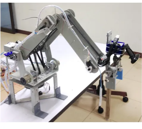
Figure 2. The robot arm structure

The image processing method is one of the important operations to find the position of the object. The object will be identified where it is by using the camera attached at the grip of the robot arm. The photo of the object taken by the camera is brought to image processing operation to separate the object from the background. The image acquisition is used to bring the image feature out from the image plane by considering the color of the object.

(3)

the object, after the object is separated from the background, the centroid command will be applied. The position of the object is then obtained in term of coordinate x and y which can be shown in Fig1

4. The Robot Arm Structure and its

Kinematics

The robot arm structure is designed to pick and place the low weight object at the desired position. It consists of 4 links connected by 4 revolute joints and the grip at the end of the robot arm. Every joint can be moved freely and their movement is independent. The dc-motors with encoder are used to drive the 4 joints and the grip which are controlled by microcontroller via RS-232 port. Its real structure is shown in Fig.2.

4.1. Forward Kinematics

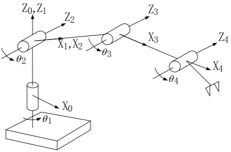
The joint relation can be described in the matrix form which the movement behaviour of the robot arm is completely described in term of the joint offset, the joint angle, the link length and the twist angle parameters. These four parameters are known as the Denavit and Hartenberg (DH) parameters [7]. The coordinate frames to define the DH parameters are shown in Fig.3 and also the DH parameters of this robot arm can be tabulated in table 1.

Z

2

Z

3

θ1 θ2

X

0

X

3

X

4

Z

4 θ3 θ4

Z ,

0

Z

1

[image:3.595.323.551.78.127.2]

X ,

1

X

2

[image:3.595.64.295.429.581.2]

Figure 3. Defining the coordinate frames on the robot arm

Table 1. Denavit – Hartenberg parameters.

link (i) αi-1 (degree) ai-1 (cm) di (cm) θi (degree)

1 0 0 12.5 θ1

2 -90 0 0 θ2

3 0 23 0 θ3

4 0 23 0 θ4

With the DH parameters evaluated in Table 1 and the calculation using forward kinematics analysis, the forward kinematics relation of the position of the manipulator of the robot arm given by 4×4 matrix can be obtained as

1 234 1 234 1 1 23 2

0 1 234 1 234 1 1 23 2

4

234 234 23 2

23 [ ]

0 23[ ] 12.5

0 0 0 1

c c c s s c c c

s c s s c s c c

s c s s

θ θ θ θ θ θ θ θ

θ θ θ θ

              − − + − + = − − − + +

T (10)

where θ234 is shorthand for θ2 + θ3 + θ4 and θ23 for θ2 + θ3. For locating the object position, the forward kinematics calculation is applied by identifying the joint angle into equation (10).

4.2. Inverse Kinematics

One approach to the inverse kinematics problem is to find the solution using algebra or geometry [8]. In this case, the joint angles are calculated using the algebraic solution technique which θ1, θ2, θ3, θ4 are in the form of the coordinate of the position x, y and z. If the position of the object in the coordinate frame are given and defined to be px,

py and pz on the x, y and z axis respectively, after using the algebraic calculation, the joint angles can be computed as in the following equations.

1

A

tan 2( , ) 180

p p

y x

θ

=

−

A

(12)

3 3 1 1

1

2 2 2

1 1

(23c 23)(12.5 ) 23s (c s )

sin

(c s ) (12.5 )

z x y

x y z

p p p

θ θ θ θ

θ θ θ − + − − − = − + −         (13)

2 2 2

1 3

25 901.75

cos

1058

x y z z

p p p p

θ

= − + + − − (14)

4 2 32 1 22 1 2 12

1 2 12 1 2 22 2 32

tan 2[s

]

,

A

r

s r

c c r

c s r

s s r

c r

θ

θ θ

θ

=

−

(15)

where r12 = -cθ1sθ234, r22 = -sθ1sθ234 and r32 = -cθ234.

5. The Robot Arm Operation

For understanding more clearly, the operation of the robot arm can be easily illustrated in the following diagram.

y_d

x, y, z _{Im age} Processing Inverse

Kinem atics θ1θ2θ3θ4

Learning Controller

Σ

desired input

+

θ1θ2θ3θ4

-Σ

u_k-1

+

u_k y_k-1

Figure 4. Block diagram of the robot arm operation

[image:3.595.317.546.559.638.2]

(4)

Cartesian coordinate which will be transformed into the relative joint angles from inverse kinematics analysis. The difference of the current and the desired joint angles is used to improve the position of the robot arm to finally reach the object.

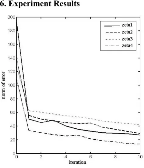
[image:4.595.57.294.163.439.2]

6. Experiment Results

[image:4.595.65.381.464.727.2]

Figure 5. The norm of error of the joint angle θ1, θ2, θ3, θ4 in 10 iterations

Figure 6. The convergence for iteration k = 100

For the experiment, the object is selected to be a

light-weight cube which its size is 6×6×6 centimeters. The object is placed somewhere in front of the robot arm within the range of the camera’s picture frame. The joints and links of the robot arm are firstly set at the initial position which all joints angles are assumed to be at 0°. Therefore, there will be the error distance between the object and the robot arm. The iteration number is chosen to be 15, 20, 50 and 100 in order to see the benefit of the iteration to the convergence. The weighting parameter for the ILC algorithm is chosen as 10-6_. The results are given in Fig.5 and Fig.6.

Fig.5 shows the behavior of the error in norm over 10 iterations. The error is the difference between the joint angles of the robot arm at the object position and at the current position of the robot arm. The graph indicates that the error in norm of the joint angle θ1,θ2, θ3, θ4 highly decreases in the first iteration. After the first iteration the errors gradually decreases in a small value as they reduce approximately by 86.13, 79.07, 67.47, and 87.45 percent respectively in the tenth iteration. The effect of the number of the iteration to the convergence is shown in Fig.6. It is seen that increasing the iteration number results in improved the convergence rates. After a hundred iteration the choice of θ1 reduces error norm by 94.96 percent.This also means that the robot arm can reach the object position more precisely.

7. Conclusions

In this paper, the use of parameter optimal iterative learning control to control the robot arm is presented. It is illustrated an observation that applying the iterative learning control with the optimization is an alternative way to successfully achieve a perfect tracking. The experimental results show that the robot arm can move progressively toward the desired target in a few iterations. The error measured from the difference between the current position of the joint angles and the target position becomes smaller every increasing the iteration. The error also decreases in the acceptable range which is within 5%. This paper suggests that the use of parameter optimal ILC algorithm does have benefits in the real work. However the additional work is needed to improve for the huge task.

REFERENCES

[1] J. W. Cheng, Y. W. Lin, and F. S. Liao, “Design and analysis of model-based iterative learning control of injection molding process,” in Proc. ANTEC 2003 Annu. Tech. Conf., Brookfield Center, CT, May, pp. 556-560.

[2] N. Amann, D. H. Owens, and E. Rogers, “Iterative learning control using optimal feedback and feedforward actions,” International Journal of Control, vol. 65, pp. 277-293, 1996. [3] S. Arimoto, S. Kawamura, and F. Miyazaki, “Bettering operations of robots by learning,” Journal of Robotic Systems, vol. 1, no. 2, pp. 123-140, 1984.

(5)

parameter optimization in high-order iterative learning contorl,” Automatica , vol. 42, pp. 287-294, 2006.

[5] D. H. Owens and J. Hatonen, “Iterative learning control – An optimiazation paradigm,” Annual Reviews in Control, 29, pp. 57-70, 2005.

[6] D. H. Owens and K. Feng, “Parameter optimization in

iterative learning control,” International Journal of Control , vol. 76, no. 11, pp. 1059-1069, 2003.

[7] S. K. Saha, Introduction to Robotics, Tata McGraw-Hill, New Delhi, 2008