Robust Controller for Vertical-Longitudinal-Lateral
Dynamics Control of Small Helicopter
Tushar K. Roy
Department of ETE, RUET, Bangladesh *Corresponding Author: [email protected]
Copyright © 2014 Horizon Research Publishing All rights reserved.
Abstract
The problem of stabilization of vertical, lateral and longitudinal dynamics for hover flight mode of an unmanned autonomous helicopter (UAH) in a gusty environment is considered. The controller design is based on a generic linear model which successfully describes the behavior of most small scale helicopters. A recursive (backstepping) design procedure is used to design the robust controller for vertical, longitudinal and lateral dynamics based on the Lyapunov’s method. For comparison purposes we design another controller based on the linear quadratic regulator (LQR) criteria. The simulation results demonstrate that the proposed controllers can effectively attenuate the gust effects and achieve rapid and accurate vertical, longitudinal and lateral position tracking when gusts occur.Keywords
Robust Backstepping Controller, LQR, External Wind Gusts, Lyapunov Function1. Introduction
Among the variety of Unmanned Air Vehicles (UAVs), unmanned autonomous helicopters constitute one of the most versatile and agile platforms for the development of autonomous flight systems. A helicopter can operate in different flight modes, such as vertical take-off/landing, hovering, longitudinal/lateral flight, and bank to turn which gives them the advantage of effective observation from various positions. Among these abilities hovering and vertical take off ability are necessarily needed. And due to their high level of agility, maneuverability and capability of operating in adverse weather conditions there are new trends of unmanned autonomous helicopter controller design nowadays. So, unmanned autonomous helicopter control system should make these performances achieved by improving the tracking performance and disturbance rejection capability. Robustness is one of the critical issues which must be considered in the control system design for small unmanned autonomous helicopter, especially those covering large flight envelope. One major problem rarely addressed by researchers to date is that of a wind disturbance.
To cope with such a problem researchers have considered approaches such as robust [9], neural network [10] etc. In this paper, we propose two controllers to stabilize the vertical, longitudinal and lateral dynamics of the small scale helicopter in the presence of wind gusts. A robust H∞ control
method of the longitudinal and lateral dynamics of the BELL 205 helicopters in the presence of model uncertainty is presented in [1]. A robust feedback method for helicopter stabilization to reject wind disturbance is presented in [2], wherein the wind disturbance is assumed to be the sum of a fixed number of sinusoids with unknown amplitudes, frequencies and phases. In [3], the authors present a robust backstepping technique of an autonomous scale helicopter subject to parameters uncertainties and uniform time varying tridimensional wind gusts. With the assistance of an unknown input observer technique (UIO), the controller is reported to be able to handle the effect of these uncertainties on the autonomous helicopter. In [4] the authors propose a nonlinear H∞ horizontal position controller for hover and
vertical external uncertainties at the same time. The main control purpose addressed here is to design the three control inputs in order to asymptotically track vertical, lateral and longitudinal references zref(t), yref(t), and xref(t), respectively.
So, this model consists of three parts with different physical backgrounds: A first subsystem describes vertical motions which are controlled by the collective pitch of the main rotor. It is strongly coupled with the torque interaction between the main rotor and the fuselage. On the other hand, forward and sideward motions, together with roll and pitch motions are controlled by lateral and longitudinal cyclic stick inputs via the flapping motion of the main rotor (second and third subsystems).
Taken into account such external wind disturbances in the model equations, we use Lyapunov’s approach to show that our proposed backstepping controller is robust with respect to external wind gusts. The performances of the controllers are simulated and tested in keeping the positions constantly in the presence of external wind gusts. The rest of this paper is organized as follows. Section (II) briefly introduces the mathematical model used and Section (III) introduces the gusts model. Section (IV) presents the control structure. Section (V) discusses simulation results. Finally, the paper concludes in Section (VI).
2. Helicopter Linear Model
Among other UAVs, Unmanned Autonomous Helicopter (UAH) has the specific characteristic; the helicopter can move vertically, float in the air, turn in place, move forward and laterally and can perform these movements in combinations. Because of this, helicopter dynamic modeling is a very complex problem. In 6DOF form, the motion states and control inputs are represented as
{
}
{
col lat lat ped}
c
u
r
p
v
q
w
u
x
δ
δ
δ
δ
φ
θ
,
,
,
,
,
,
,
,
,
,
=
=
The variables u, v and w represent the helicopter linear
velocity in body frame; p, q and r denote roll, pitch and yaw rates respectively; and
φ
, θ represent roll, pitch attitude respectively. A conventional single main rotor helicopter has four independent control inputs,δ
lat,δ
lon,δ
col andδ
ped which denote the deflection of the lateral cyclic, longitudinal cyclic, main rotor collective pitch and tail rotor collective pitch respectively. The collective commands control the magnitude of the main rotor and tail rotor thrust and other two control commands control the inclination of the Tip-Path-Plane (TPP) on the longitudinal and lateral direction.Before getting into the control law design longitudinal and lateral dynamics should be analyzed. For this purpose, the nonlinear form of a helicopter equations of motion are given as follows,
m
X
g
wq
vr
u
=
(
−
)
−
sin
θ
+
(1)m
Y
g
ur
wp
v
=
(
−
)
+
sin
φ
cos
θ
+
(2)m
Z
g
vp
uq
w
=
(
−
)
+
cos
φ
cos
θ
+
(3)xx xx
zz yy
I
L
I
I
I
qr
p
=
(
−
)
+
(4)yy yy
xx zz
I
M
I
I
I
pr
q
=
(
−
)
+
(5)zz zz
yy xx
I
N
I
I
I
pq
r
=
(
−
)
+
(6)where, where, forces [X,Y,Z]' and moments [L,M,N]' are expressed in the body frame, m is the helicopter mass and Ixx,
Iyy and Izz are the moment of inertial about x, y, and z axis. In
order to complete the system, we need to the following two equations which relate the Euler angle rates to the angular velocity [7].
θ
φ
θ
φ
φ
=
p
+
q
sin
tan
+
r
cos
tan
(7)φ
φ
θ
=
q
cos
−
r
sin
(8) We know that the cyclic longitudinal and lateral tilt of the main rotor disk is controllable through the cyclic pitch. Therefore, in this model, the longitudinal and lateral flapping dynamics can be represented by the first order equations as follows [8]:)
(
1
1
1
q
a
u
a
u
A
lon lona
δ
τ
τ
∂
+
∂
+
−
−
=
(9))
(
1
1
1
p
b
u
b
v
A
lat latb
δ
τ
τ
∂
+
∂
+
−
−
=
(10)where,
δ
latandδ
lonare the lateral and longitudinal cyclic control inputs, a1 and b1 are the lateral and longitudinalflapping angles and Alon and Blat are effective steady-state
longitudinal and lateral gains from the cyclic inputs to the main rotor flapping angles. In Eqn. (9) and Eqn. (10),
u
a
A
u∂
∂
=
1 andv
b
B
v∂
∂
=
1 are constants and represent the longitudinal and lateral Dihedral effect. The dihedral effect is the change of tip-path-plane (TPP) tilt due to the longitudinal and lateral velocities [16]. The Dihedral effect is modeled by the following equation)
2
8
(
2
1
1 T T
b
C
a
C
R
v
b
u
a
+
Ω
=
∂
∂
−
=
∂
∂
σ
where, Rb is the main rotor radius, σ solidity ratio, ‘a’ lift
curve slope and CT thrust coefficient. Since the rotor is
symmetric, we consider Au=-Bv.
Linearization is essential to derive simplified working models, considering inherent instability under hover and slow flight conditions. So, after linearizing equations (Eq. 1-8) we get following parameterized model of decoupled longitudinal and lateral dynamics.
lon lon u
a q
u
a q
u
A a
q u
A
M M
M
X g X X
a q u
δ
τ
θ
τ
τ
θ
+
− −
−
=
0 0 0
1 0 1
0 0 1 0
0
1 1
(11)
lat
lat v
b p
v
b p
v
A b
p v
B
L L
L
Y g Y Y
b p v
δ
τ φ τ τ
φ
+
− −
=
0 0 0
1 0 1
0 0 1 0
0
1 1
(12)
where
u
M
I
M
u
X
m
X
yy u
u
∂
∂
=
∂
∂
=
1
,
1
... are the force and moment derivatives normalized by the mass of the helicopter or respective moment of inertia. The pitching flap-stiffness constant is represents by Ma that can be computed as follows[17]:
yy yy
z
a
I
K
I
mM
M
=
+
βwhere Mz is the height of the
rotor hub above the fuselage center of gravity, Iyy is the
pitching moment of inertia and Kβ is the rotor blade spring
stiffness. Similarly the lateral flap-stiffness constant Lb can
be computed as follows:
xx xx
z
b
I
K
I
mM
L
=
+
β.
The proposed linear model has been successfully adopted for control applications in a large number of small-scale unmanned helicopters [18-26]. In order to stabilize and control the helicopter system for longitudinal and lateral dynamics, we use robust backstepping controller.
Remark 1: Control inputs in the controller design process are set to be longitudinal and lateral flapping angles. They will be converted later into longitudinal cyclic and lateral cyclic for implementation.
B. Formation of Vertical Dynamics
Since we are also interested to control the altitude so, we need to express the equation (3) i.e. z dynamics in earth frame. To this end, we use the rotation matrix between the body and earth frames and obtain the following altitude dynamics:
m
Z
g
w
=
+
(cos
φ
cos
θ
)
(13) Altitude dynamics can be linearized around hover conditions, i.e.,φ
≈
0
,
θ
≈
0
,
andψ
≈
0
. So, resulting linearized altitude dynamics can be expressed in the earth frame asm
T
mg
w
=
−
(14)
3. Gust Model
The purpose of including wind gusts into the simulation model is to ensure that the design controller can cope with a real-world environment where wind effects can be a significant challenge to station keeping. For analyses of RUAV, wind gusts can be treated as either random (spectral turbulence) or discrete. For random gusts, typical spectral models include the Von Karman and Dryden turbulence models. The Von Karman model has widely been considered the more "realistic" model when it comes to defining turbulence spectra. However, due to the computational complexity of the Von Karman model, the Dryden model is typically used in aerospace vehicle analyses. There are many sources for wind models based upon empirical data that consist of passing band limited white noise through appropriate forming filters. The turbulence models are scaled with respect to RUAV altitude, velocity, wing span. Vertical wind gusts can be neglected compared with its horizontal counterparts due to small quantity component. Consequently we consider the horizontal wind gusts model in this work, and corresponding forming filters including Hu(s) for
longitudinal direction and Hv(s) for lateral direction, take the
following transfer function forms,[11] respectively:
s
U
L
U
L
s
H
u u u u
+
=
1
1
2
)
(
π
σ
2
1
3
1
)
(
+
+
=
s
U
L
s
U
L
U
L
s
H
v v u
v
v
σ
π
2
1
3
1
)
(
+
+
=
s
U
L
s
U
L
U
L
s
H
w w w
v
w
σ
π
where, U is the true speed of a RUAV, σu, and σv are the root
mean square intensities of the turbulence and Lu, and Lv are
the turbulence scale lengths that describe the behavior of the wind gusts. In this work, the scale of turbulence, Lu, and Lv
are assigned constant values of Lu= Lv=722.5m. And for low
altitude region (altitude < 1000ft) the σu, σv, and σw
turbulence intensities are given by 20
1
.
0
W
w
=
4 . 0
)
000823
.
0
177
.
0
(
1
h
wv w u
+
=
=
σ
σ
σ
σ
(16)
where, W20 is the wind speed at 20 ft (6m) above the ground
and can be approximated by U and altitude is described by h. In this paper, we have considered a typical wind speed of 10
m/s and an altitude of 2 m.
4. Controller Design
In this section, we design the controller for the Vertical, longitudinal and lateral dynamics of the helicopter dynamics separately and each based on an appropriate decoupled model. And for that a robust backstepping control method-based on Lyapunov’s function for the position stabilize of a small scale helicopter is presented through the control of longitudinal and lateral flapping angles and collective pitch as the control inputs. But for comparison purposes we also design another controller based on the linear quadratic regulator (LQR) criteria. The linear motion equations for longitudinal and lateral dynamics are described through Eq. (11-12). In the longitudinal dynamics (11), the parameter a1
is a function of u and q. Similarly in the lateral dynamics (12), the parameter b1 is a function of v and p. Hence, we
cannot carry out the flight control laws via backstepping considering a1 and b1 as the control input. A common
simplification practice, presented in [6] is to neglect the effect of the lateral and longitudinal forces produced by the flapping angles. These parasitic forces have a minimal effect on the translational dynamics compared to the propulsion forces produced by the stability derivatives
X
θ andX
φ(in (11) and (12) are denoted by −g and g, respectively). We
also neglect the stability derivative terms Xq and Yp for
deriving controller, because they are much smaller than the propulsion forces produced by the stability derivatives
X
θand
X
φ This assumption is physically meaningful andresults into a linear system in feedback form.
According to our design purposes the helicopter should be separated into two interconnected subsystems. The first subsystem accounts for longitudinal mode and second subsystem accounts for lateral mode. As indicated in the above, the effect of the translational forces produced by the flapping motion of the main rotor is parasitic and negligible compared to the main source of propulsion, which are the forces produced by the roll and pitch attitude change of the fuselage. By neglecting the effect of the parameters Xa , Yb,
Xq and Yp the longitudinal-lateral dynamics will have strict
feedback forms. As a result the simplified description of the longitudinal mode is given as follows,
u
x
=
,u
=
X
uu
−
g
θ
q
=
θ
,q
=
M
uu
+
M
qq
+
M
aa
1 Similarly the simplified description of the lateral mode isgiven as,
v
y
=
,v
=
Y
vv
+
g
φ
p
=
φ
,p
=
L
vv
+
L
pp
+
L
bb
1 A. Longitudinal DynamicsIn this subsection, the robust backstepping controller based on Lyapunov method is designed for the longitudinal dynamics in the presence of wind gusts. Linear model equations of the longitudinal dynamics under external disturbance are rewritten as:
u
x
=
,u
=
X
uu
−
g
θ
,θ
=
q
A
a
M
q
M
u
M
q
=
u+
q+
a 1+
where,A
is an unknown parameter which is estimated asA
ˆ
. The estimation error onA
is assumed bounded by known constant F, that is,A
−
A
ˆ
≤
F
Step1: The design process starts with the definition of the longitudinal position error i.e.,
t
x
z
u
x
z
x
x
z
1=
−
d,
1=
−
d,
1=
(17) We consider u as a virtual control input and define ud as avirtual control law for Eqn. (17). Let z2 be an error variable
representing the difference between the actual and virtual control inputs i.e.,
d
d
u
z
u
u
u
z
2=
−
,
=
2+
Therefore, . At this stage we would like to design a virtual control law ud which would make
z
1→
0
as∞
→
t
Consider a control Lyapunov function 21
1
2
1
z
W
=
And its derivative as follows,
)
(
,
1 1 2 11
1
z
z
W
z
z
u
dW
=
=
+
We can now select an appropriate virtual control law ud
which would make
W
1≤
0
. A possible choice is1 1
z
k
u
d=
−
then,2 1 2 1 1
1
k
z
z
z
W
=
−
+
. Clearly ifz
2=
0
then0
2 1 1
1
=
−
k
z
≤
W
.where, k1 is a scalar parameter which can be used to tune the
output response. Now consider the time derivative of ud as
1 1
z
k
u
d=
−
,u
d=
−
k
1u
(18) Step2: We derive the error dynamics forz
2=
u
−
u
d and its time derivative as follows,d
u
u
In which θis viewed as a virtual control input. Now define a virtual control law
θ
dand let z3 be an error variablerepresenting the difference between actual and virtual controls i.e.,
z
3=
θ
−
θ
d)
(
)
(
1 32
x
uk
u
g
z
dz
=
+
−
+
θ
Now choose a control Lyapunov function as follows, 2
2 1
2
W
1
2
z
W
=
+
. And its derivative as follows,3 2 1 1 2 2 1 1 2 2 2 1 2
}
)
(
{
z
x
k
u
g
gz
z
z
z
k
W
z
z
W
W
du
+
−
−
+
+
−
=
+
=
θ
We can now select an appropriate virtual control
θ
d to cancel out some terms related to z1, z2and u, while the terminvolving z3 cannot be removed.
}
)
(
{
1 1 2 21
z
x
k
u
k
z
g
ud
=
−+
+
+
θ
Therefore,
W
2=
−
k
1z
12−
k
2z
22−
gz
2z
3.Clearly if
z
3=
0
then 20
2 2 2 1 1
2
=
−
k
z
−
k
z
≤
W
.Now the time derivative of
θ
dis}
)
(
{
1 1 2 21
z
x
k
u
k
z
g
ud
=
−+
+
+
θ
}
)
)(
(
{
1 2 21
u
x
k
x
u
g
k
z
g
u ud
=
−+
+
−
θ
+
θ
Step3: We derive the error dynamics for
z
3=
θ
−
θ
d.And its time derivative as follows,
z
3=
θ
−
θ
d)}
(
)
{(
)}
)(
(
{
3 1 2 1 1 1 3 d u u uz
g
u
k
x
k
g
g
u
x
k
x
u
g
q
z
θ
θ
+
−
+
−
−
+
+
−
=
− −
In which q is viewed as a virtual control input. Now define a virtual control law qd and let z4 be an error variablerepresenting the difference between actual and virtual control input i.e.,
z
4=
q
−
q
dTherefore,
)}
(
)
{(
)}
)(
(
{
3 1 2 1 1 1 4 3 d u u u dz
g
u
k
x
k
g
g
u
x
k
x
u
g
q
z
z
θ
θ
+
−
+
−
−
+
+
−
+
=
− −
Now choose a control Lyapunov function , 2
3 2
3
W
1
2
z
W
=
+
. And its time derivative as follows,3 3 2
3
W
z
z
W
=
+
)}]
(
)
{(
)}
)(
(
{
[
3 1 2 1 1 1 4 3 2 3 2 2 2 2 1 1 3 d u u u dz
g
u
k
x
k
g
g
u
x
k
x
u
g
q
z
z
z
gz
z
k
z
k
W
θ
θ
+
−
+
−
−
+
+
−
+
+
−
−
−
=
− −
We can now select an appropriate virtual control qd to
cancel out some terms related to z1, z2, z3 and u, while the
term involving z4 cannot be removed.
3 3 3 1 2 1 1 1 2
)}]
(
)
{(
)}
)(
(
{
z
k
z
g
u
k
x
k
g
g
u
x
k
x
u
g
gz
q
d u u u d−
+
−
+
+
−
+
+
+
=
− −θ
θ
And its derivative as follows,
3 3 3 1 2 1 1 1 2
)}]
(
)
{(
)}
)(
(
{
z
k
z
g
u
k
x
k
g
g
u
x
k
x
u
g
z
g
q
d u u u d
−
+
−
+
+
−
+
+
+
=
− −θ
θ
Suppose,
q
d=
f
(
z
2,
z
3,
u
,
θ
,
θ
d)
Therefore,
W
3=
−
k
1z
12−
k
2z
22−
k
3z
32+
z
3z
4 . Clearly if0
4
=
z
thenW
3=
−
k
1z
12−
k
2z
22−
k
3z
32≤
0
Step4: We derive the error dynamics forz
4=
q
−
q
d.And its derivative as follows,
)
,
,
,
,
(
,
3 2 1 4 4 d a q u du
z
z
f
A
a
M
q
M
u
M
z
q
q
z
θ
θ
−
+
+
+
=
−
=
In the above equation the actual control input appears. Our objective is to design the actual control input ‘a1’ such that z1,
z2, z3, and z4 converge to zero as t→∞.
Choose a Lyapunov function W4 as, 4 3 42
2
1
z
W
W
=
+
.And its time derivative as follows,
))
,
,
,
,
(
(
1 2 34 4 3 2 3 3 2 2 2 2 1 1 4 4 4 3 4 d a q
u
u
M
q
M
a
A
f
z
z
u
M
z
z
z
z
k
z
k
z
k
W
z
z
W
W
θ
θ
−
+
+
+
+
+
−
−
−
=
+
=
We are finally in the position to design control ‘a1’ by
making
W
4≤
0
as follows,))
sgn(
)
,
,
,
,
(
ˆ
(
4 4 4 3 2 3 1 1z
F
z
k
u
z
z
f
A
q
M
u
M
z
M
a
d q u a+
+
−
+
+
+
−
=
−θ
θ
(19)Therefore,
0
))
sgn(
ˆ
(
4 4 2 4 4 2 3 3 2 2 2 2 1 1 4≤
−
−
+
−
−
−
−
=
z
F
A
A
z
z
k
z
k
z
k
z
k
W
B. Lateral Dynamics
as:
y
=
v
,v
=
Y
vv
+
g
φ
,p
=
φ
,p
=
L
vv
+
L
pp
+
L
bb
1+
δ
where,
δ
is an unknown parameter which is estimated asδ
ˆ
. The estimation error onδ
is assumed bounded by known constant Fl, that is,δ
−
δ
ˆ
≤
F
l.Step1: The design process starts with the definitionof the lateral position tracking error i.e.,
v
e
y
y
e
y
y
e
1=
−
d,
1=
−
d,
1=
(20) We consider v as a virtual control input and define vdvirtual control law for Eqn.(20). Let e2 be an error variable
representing the difference between the actual and virtual control inputs i.e.,
,
,
22
v
v
dv
e
v
de
=
−
=
+
Therfore,
e
1=
e
2+
v
dAt this stage we would like to design a virtual control law
vd which would make
e
1→
0
ast
→
∞
. Consider a control Lyapunov function, 1 122
1
e
W
=
And its time derivative as follows,
)
(
,
1 1 2 11
1
e
e
W
e
e
v
dW
=
=
+
We can now select an appropriate virtual control vdwhich
would make
W
1≤
0
.A possible choice isv
d=
−
c
1e
1 then2 1 2 1 1
1
c
e
e
e
W
=
−
+
. Clearly if e2=0 thenW
1=
−
c
1e
12≤
0
where, c1 is a scalar parameter which can be used to tunethe output response. Now consider the time derivative of vd
as,
v
c
v
e
c
v
d=
−
1
1,
d=
−
1 Step2: We derive the error dynamics fore
2=
v
−
v
dand itsderivative as follows,
v
c
g
v
Y
e
e
c
g
v
Y
e
v
v
e
2=
−
d,
2=
v+
φ
+
1
1,
2=
v+
φ
+
1 In whichφ
is viewed as a virtual control input. Now define a virtual control lawφ
d and let e3 be an error variablerepresenting the difference between the actual and virtual control inputs i.e.,
e
3=
φ
−
φ
dTherefore,
e
2=
(
Y
v+
c
1)
v
+
g
(
e
3+
φ
d)
. Now choose a control Lyapunov function2 2 1
2
W
1
2
e
W
=
+
And its derivative as,
2 2 1
2
W
e
e
W
=
+
3 2 1 1 2 2 1 1
2
c
e
e
{
e
(
Y
c
)
v
g
}
ge
e
W
=
−
+
+
v+
+
φ
d+
We can now select an appropriate virtual control
φ
d to cancel out some terms related to e1, e2 and v, while the terminvolving e3 cannot be removed.
}
)
(
{
1 1 2 21
e
Y
c
v
c
e
g
vd
=
−
−+
+
+
φ
Therefore,
W
2=
−
c
1e
12−
c
2e
22+
ge
2e
3 , clearly if0
3
=
e
then 22 2 2 1 1
2
c
e
c
e
W
=
−
−
. Now the timederivative of
φ
d}
)
)(
(
{
}
)
(
{
2 2 1 1 2 2 1 1 1e
c
g
v
Y
c
Y
v
g
e
c
v
c
Y
e
g
v v d v d
+
+
+
+
−
=
+
+
+
−
=
− −φ
φ
φ
Step3: We derive the error dynamics fore
3=
φ
−
φ
d. And its derivative as follows,)}
(
)
{(
)}
)(
(
{
3 1 2 1 1 1 3 3 d v v v de
g
v
c
Y
c
g
g
v
Y
c
Y
v
g
p
e
e
φ
φ
φ
φ
+
+
+
+
+
+
+
+
=
−
=
− −
In which p is viewed as a virtual control input. Now define a virtual control law pd and let e4 be an error variable
representing the difference between actual and virtual controls i.e.,
d
d
p
e
p
p
p
e
4=
−
,
=
4+
)}
(
)
{(
)}
)(
(
{
3 1 2 1 1 1 4 3 d v v v de
g
v
c
Y
c
g
g
v
Y
c
Y
v
g
p
z
e
φ
φ
+
+
+
+
+
+
+
+
+
=
− −
Now choose a control Lyapunov function
2
1 2
3 2
3 W e
W = +
And its derivative as,
3 3 2
3
W
e
e
W
=
+
)]
(
)
{(
)}
)(
(
{
[
3 1 2 1 1 1 4 3 2 3 2 2 2 2 1 1 3 d v v ve
g
v
c
Y
c
g
g
v
Y
c
Y
v
g
p
e
e
e
ge
e
c
e
c
W
φ
φ
+
+
+
+
+
+
+
+
+
+
+
−
−
=
− −
We can now select an appropriate virtual control pd to
cancel some terms related to e1, e2, e3 and v, while the term
involving e4 cannot be removed.
3 3 3 1 2 1 1 1 2
)]
(
)
{(
)}
)(
(
{
e
c
e
g
v
c
Y
c
g
g
v
Y
c
Y
v
g
ge
p
d v v v d−
+
+
+
−
+
+
+
−
−
=
− −φ
φ
And its derivative as follows,Suppose,
p
d=
f
(
e
2,
e
3,
v
,
φ
,
φ
d)
Therefore,W
3=
−
c
1e
12−
c
2e
22−
c
3e
32+
e
3e
4. Clearlyif
0
4
=
e
then 20
3 3 2 2 2 2 1 1
3
=
−
c
e
−
c
e
−
c
e
≤
W
Step4: We derive the error dynamics for
e
4=
p
−
p
dand its time derivative as,
)
,
,
,
,
(
2 3 1 4 4 d b p v dv
e
e
f
b
L
p
L
v
L
e
p
p
e
φ
φ
δ −
+
+
+
=
−
=
(19) In the above equation (17) the actual control input appears. Our objective is to design the actual control input ‘b1’ suchthat e1, e2, e3, and e4 converge to zero as t→∞. Choose a
Lyapunov function W4 as, 4 3 42
2
1
e
W
W
=
+
and itsderivative as follows,
W
4=
W
3+
e
4e
4))
,
,
,
,
(
(
1 2 34 4 3 2 3 3 2 2 2 2 1 1 4 d b p
v
v
L
p
L
b
f
e
e
v
L
e
e
e
e
c
e
c
e
c
W
φ
φ
δ
−
+
+
+
+
+
−
−
−
=
We choose our control input b1 as follows,
)) sgn( ) , , , , ( ˆ ( 4 4 4 3 2 3 1 1 e F e c v e e f p L v L z L b d p v b + + − + + + − = − φ φ
δ (21)
Then, 0 )) sgn( ˆ ( 4 4 2 4 4 2 3 3 2 2 2 2 1 1 4 ≤ − − + − − − − = e F e e c e c e c e c W δ δ
(22)
C. Vertical Dynamics
In this subsection, a nonlinear robust backstepping controller for helicopter altitude stabilization in the presence of external wind gusts is designed based on Lyapunov function. The vertical dynamics is dependent on the vertical altitude z and the collective pitch,
θ
0. We know the altitude zis controlled by T through collective pitch
θ
0. So, vertical dynamics motion equations of the helicopter are written as follows:w
z
=
ε
+
−
=
m
T
mg
w
(23)where, ε is an unknown parameter but estimated as
ε
ˆ
. The estimation error on ε is assumed bounded by known constant Fv, that is ε−εˆ ≤Fv.Step 1: The design process starts with the definition of the altitude tracking error and its derivative as follows:
w
e
z
e
z
z
e
1=
−
0,
1=
,
1=
(24) We view w as a virtual control input for equation (14) anddefine wd is the virtual control law. Let e2 be an error variable
representing the difference between the actual and virtual control of (24) i.e.,
e
2=
w
−
w
d,
w
=
e
2+
w
dTherefore,
e
1=
e
2+
w
dIn this step our control objective is to design a virtual control law wd which would make e1→0 as
t
→
∞
.Now consider a control Lyapunov function, 1 12
2
1
e
V
=
,whose time derivative as follows,
)
(
,
1 1 2 11
1
e
e
V
e
e
w
dV
=
=
+
We can now select an appropriate virtual control wdwhich
would make
V
1≤
0
.A possible choice is
w
d=
−
α
e
1 (25) where, α is a scalar parameter which can be used to tune the output response.Therefore,
V
1=
−
α
e
12+
e
1e
2Clearly if
e
2=
0
, thenV
1=
−
α
e
12≤
0
.Now time derivative of the equation (24) as follows,
,
2
w
w
de
=
−
w
m
T
g
e
2=
−
+
ε
+
α
(26)Again we know,
+
−
′
Ω
=
ρ
θ
µ
λ
2
1
)
2
3
1
(
3
2
)
(
R
2A
b 0 2a
T
where,.
)
(
ˆ
2
ˆ
2
2
ˆ
,
,
)
(
,
,
2 2 2 2 2 2 2 2 2 1 1 t n t i t z s n t n iv
v
v
v
v
A
T
v
v
v
u
v
v
v
b
u
i
a
v
R
v
R
v
v
+
+
=
−
+
=
+
=
−
−
+
=
Ω
=
Ω
+
=
′
ρ
µ
λ
Now, by substituting the value of T into Eqn. (27) we get,
w
m
B
m
B
g
e
=
−
θ
+
µ
+
λ
′
+
ε
+
α
2
)
2
3
1
(
3
2 0 2
where,2
)
(
2 bA
R
a
In the above equation the actual control input appears. Our objective is to design the actual control input
θ
0 such thate1 and e2 converge to zero. Now choose a Lyapunov function
V2 as follows,
2 2 1
2
V
2
1
e
V
=
+
And its time derivative as follows,
2 2 1
2
V
e
e
V
=
+
}
2
)
2
3
1(
3
{
0 22 2 1 2 1
2
e
e
e
e
g
B
m
B
m
w
V
=
−
α
+
+
−
θ
+
µ
+
λ
′
+
ε
+
α
} 2
) 2 3 1( 3
{ 0 2
1 2 2 1
2 e e e g Bm Bm w
V =−
α
+ + −θ
+µ
+λ
′+ε
+α
We choose our control input θ0 as follows,
+ +
+ + ′ + +
+ =
) ( sgn
ˆ 2
) 2 3 1 (
3
2 2
1
2 0
e F e
w m
B g e B
m
v β
α ε λ µ
θ (28)
Then
}
2
))
sgn(
ˆ
2
(
{
2 2
1 1
2 2 1 2
w
m
B
e
F
e
w
m
B
g
e
g
e
e
e
V
v
λ
ε
α
β
ε
α
λ
α
+
+
′
+
+
+
+
+
′
+
+
−
+
+
−
=
2
(
ˆ
sgn(
2))
0
2 2 2 1
2
=
−
e
−
e
+
e
−
−
F
e
≤
V
α
β
ε
ε
v (29)D. LQR Controller Design
Linear quadratic regulator (LQR) controller is considered as one of the most important state space based optimal control methods. In LQ problem, the system dynamics are described by a set of linear differential equations and its cost is described by a quadratic function. The solution for the problem is provided by the linear-quadratic regulator. LQR theory results in a linear control law which minimizes the integral over an infinite time interval of the weighted sum of the squares of the elements of the system state and control vectors. Consider the linear time-invariant system
x
C
y
u
B
x
A
x
=
+
=
(30)
wherein the state
x
∈
ℜ
n, the input controlu
∈
ℜ
m, and the measured outputy
∈
ℜ
p . To design the LQR controller, the first step is to select the weighting matrices Q and R, where Q is weighting factors that weight the states and R is also weighting factors that weights inputs. Then the feedback K can be computed and the closed loop systemresponses can be found by simulation. The sate feedback control law has the form:
x
K
u
=
−
(31) where K is am
×
n
matrix which minimizes the following performance matrix:dt
Ru
u
x
Q
x
J
T T∫
∞+
=
0
(
)
(32)In (32), Q and R are the positive definite (or positive semi-definite) weighting matrices which will balance the relative importance of the input and state in the cost function
J that we are trying to optimize. The state feedback gain can be computed as follows,
P
B
R
K
=
−1 Twhere P is a positive definite matrix obtained from the solution of the following algebraic Riccati equation:
0
1
=
−
+
+
PA
Q
PBR
−B
P
P
A
T T (33)5. Simulation Results
In this section, robust backstepping control and LQR are now compared via simulations. Simulation is conducted for the case in which the initial positions are set to x = 0 m , y = 0 m and z=-2 m and its desired positions to x = 0 m, y = 0 m and z=2 m. The roll angle trim ϕref is initialized at 4.50 to
compensate for the tail rotor thrust. The effectiveness of the proposed controlleris investigated in a gusty environment by comparing it with the LQR controller.In order to determine
F, Fl and Fvat first we set up a mean velocity of the wind
gusts and found the pitch rate, roll rate and vertical acceleration response. Again we set up another mean velocity of the wind gusts and found the pitch rate, roll rate and vertical acceleration response. From thesetwo results we found the pitch rate, roll rate vertical acceleration variation due to the external windgusts. From these pitch rat, roll rate and vertical acceleration variation we set up the bound constants are to be F = 0.5 deg/s, Fl = 0.4 deg/s and Fv=0.8
m/s2 on the basis of pitch rate, roll rate vertical acceleration
variation respectively for external wind gusts. The weighting matrices for both longitudinal and lateral modes are considered to be Qlon=diag[0.1 0.1 0.5 0.6], Rlon=30 and
Qlat=[0.5 0.01 0.5 0.6], Rlat=80 respectively. The state
feedback matrices for both longitudinal and lateral dynamics are Klon=[-0.1421 0.1043 0.6046 -0.1414] and Klat=[0.1169
Figure 1. Helicopter position response using backstepping and LQR Controller
Fig. 1 shows the performances of the proposed robust backstepping controller (blue line) and LQR controller (green line) and it is clear from the simulation results that the position tracking error is almost zero for robust backstepping controller but relatively large for the LQR controller.
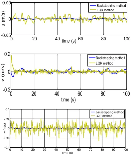
Figure 2. Helicopter velocity response using backstepping and LQR
controller
Figure 3. Helicopter orientation response using backstepping and LQR
controller
Figure 4. Helicopter roll rate response using backstepping and LQR
controller
Figure 5. Helicopter pitch rate response using backstepping and LQR
controller
Figure 6. Helicopter yaw rate response using backstepping and LQR
controller
0 10 20 30 40 50 60 70 80 90 100
1.9 1.95 2 2.05 2.1
time (s)
Z (
m)
Backstepping method LQR method
0 20 40 60 80 100
-0.05 0 0.05
time (s)
u
(m/
s)
Backstepping method LQR method
0 20 40 60 80 100
-0.2 0 0.2
time (s)
v
(
m/
s
)
Backstepping method LQR method
0 10 20 30 40 50 60 70 80 90 100
-0.1 -0.05 0 0.05 0.1
time (s)
w
(m/
s)
Backstepping method LQR method
0 20 40 60 80 100
0 2 4 6 8
time (s)
R
ol
l an
gl
e
(de
g) Backstepping method
LQR method
0 20 40 60 80 100 -0.5
0 0.5
time (s)
P
itc
h
ang
le
(
deg
)
Backstepping method LQR method
0 10 20 30 40 50 60 70 80 90 100
-10 -5 0 5 10
time (s)
Yaw
angl
e (
deg)
Backstepping method LQR method
0 20 40 60 80 100
-5 0 5
time (s)
R
ol
l r
at
e
(de
g/
s) Backstepping method
LQR method
0 20 40 60 80 100
-1 0 1
time (s)
Pi
tc
h
ra
te
(d
eg
/s
) Backstepping method
LQR method
0 10 20 30 40 50 60 70 80 90 100
-20 -10 0 10 20
time (s)
Yaw
rat
e (
deg/
s)
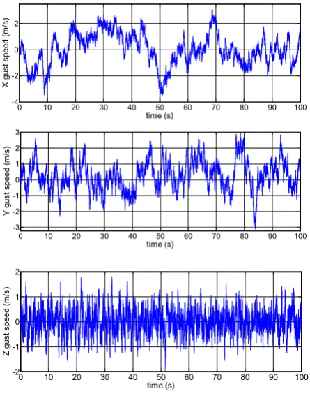
[image:9.595.64.293.82.329.2] [image:9.595.319.543.365.429.2] [image:9.595.72.283.434.682.2] [image:9.595.313.547.467.535.2] [image:9.595.316.544.576.660.2]Figure 7. Wind gusts to test controller
The faster responses are the outcome of the rapid velocity responses depicted in Fig.2 and it is clear that velocities are converged quickly to zero with smaller excursions and smaller fluctuation unlike LQR controller. The roll, pitch and yaw angles of both controllers are presented in Fig. 3. For the robust backstepping controller, the roll angle settles approximately within the desired value (4.50), but for the
LQR controller, it settles in the range of 2.50 to 3.950. Fig. 4,
Fig. 5, and Fig.6, shows the roll, pitch and yaw rates of the small Vario XLC helicopter which are almost zero for the robust backstepping controller while the oscillations are not damped completely for the LQR controller. Therefore it is clear that the proposed robust backstepping controller is better than the LQR controller in a gusty environment. The Dryden wind disturbance is shown in fig.7 that used in the simulation to test the controllers.
6. Conclusion
In this paper, a Lyapunov’s based backstepping control and LQR control have been applied for the control of longitudinal, lateral and vertical position of the small scale helicopter in the presence of wind gusts. Comparison simulation results show that the robust backstepping controller can settle the longitudinal, lateral and vertical position of the small helicopter more rapidly than an LQR controller in a gusty environment. Considering the simulation performed, LQR controller also successful to stabilize the longitudinal, lateral and vertical position of the helicopter but as seen by the fact that helicopter cannot hover
at the desired position (x=0 m, y=0 m and z=2 m). Even for large external disturbances, the proposed backstepping controller is robust against this external disturbance. So, our propose backstepping controller better than LQR controller in a gusty environment. But we can say that the two proposed controls algorithm produces satisfactory performances. Implementation of our proposed autonomous flight control method on the real system and flight test to prove its feasibility in real applications are remained for future work.
REFERENCES
[1] D.J.Wallcer, M.C. Turner, AJ. Smerlas, ME. Strange, and A.W. Gubbels, “Robust Control of the Longitudinal and Lateral Dynamics of the BELL 205 Helicopter,” Proceedings of the American Control Conference San Diego, California June 1999.
[2] Kumeresan A. Danapalasingam, John-Josef Leth, Anders la Cour-Harbo and Morten Bisgaard “Robust Helicopter Stabilization in the Face of Wind Disturbance” 49th IEEE Conference on Decision and Control, December 15-17, 2010 Hilton Atlanta Hotel, Atlanta, GA, USA.
[3] T. Cheviron, F. Plestan, and A. Chriette, “A robust guidance and control scheme of an autonomous scale helicopter in presence of wind gusts,” International Journal of Control, Vol. 82, No. 12 December 2009, 2206-2220.
[4] Xilin Yang, Matt Garratt, and Hemanshu Pota, “ A Nonlinear Position Controller Operations of Rotary-wing UAVs,” 18th IFAC World Congress Milano (Italy) August 28- September 2, 2011.
[5] T. Cheviron, F. Plestan, and A. Chriette, “A robust guidance and control scheme of an autonomous scale helicopter in presence of wind gusts,” International Journal of Control, Vol. 82, No. 12 December 2009, 2206-2220.
[6] Ioannis A. Raptis and Kimon P. Valavanis, “Velocity and Heading Tracking Control For Small-Scale Unmanned Helicopters” American Control Conference on O'Farrell Street, San Francisco, CA, USA June 29 - July 01, 2011. [7] D. McLean. Automatic Flight Control Systems. Prentice
Hall, 1990
[8] M. Garratt. Biologically inspired vision and control for an autonomous flying vehicle. PhD thesis, Austarlian National University, October 2007.
[9] T. Cheviron, F. Plestan and A. Chriette,”A robust guidance and control scheme of an autonomous scale helicopter in presence of wind gusts”,International Journal of Control, Vol. 82, No. 12, December 2009, 2206-2220.
[10] L. Guo, C. Melhuish, and Q. Zhu, “Towards neural adaptive hovering control of helicopters,” in Proc. IEEE Int. Conf. Control Applications, Glasgow, U.K., Sep. 2002 , pp. 54-58. [11] N. C. Nigam and S. Narayanan, “Application of Radom
Vibration”, Springer-Verlag, New Delhi, 1994.
[12] S. Suresh, P. Kashyab and M. Nabi, “Automatic Take-off Control System for Helicopter –An H∞ Apporach,” 11th
0 10 20 30 40 50 60 70 80 90 100
-4 -2 0 2
time (s)
X
gus
t s
peed
(m
/s
)
0 10 20 30 40 50 60 70 80 90 100
-3 -2 -1 0 1 2 3
time (s)
Y
gus
t s
peed
(m
/s
)
0 10 20 30 40 50 60 70 80 90 100
-2 -1 0 1 2
time (s)
Z
gus
t s
peed
(m
/s