Aspects of solar wind interaction with Mars: comparison of fluid and hybrid simulations

www.ann-geophys.net/25/145/2007/ © European Geosciences Union 2007

Annales

Geophysicae

Aspects of solar wind interaction with Mars: comparison of fluid

and hybrid simulations

N. V. Erkaev1, A. B¨oßwetter2, U. Motschmann2, and H. K. Biernat3

1_{Institute for Computational Modelling, Russian Academy of Sciences, 660036, Krasnoyarsk, Russia} 2_{Institute for Theoretical Physics, TU Braunschweig, Germany}

3_{Space Research Institute, Austrian Academy of Sciences, Graz, Austria}

Received: 9 May 2006 – Revised: 11 October 2006 – Accepted: 10 January 2007 – Published: 1 February 2007

Abstract. Mars has no global intrinsic magnetic field, and consequently the solar wind plasma interacts directly with the planetary ionosphere. The main factors of this interac-tion are: thermalizainterac-tion of plasma after the bow shock, ion pick-up process, and the magnetic barrier effect, which re-sults in the magnetic field enhancement in the vicinity of the obstacle. Results of ideal magnetohydrodynamic and hybrid simulations are compared in the subsolar magnetosheath re-gion. Good agreement between the models is obtained for the magnetic field and plasma parameters just after the shock front, and also for the magnetic field profiles in the magne-tosheath. Both models predict similar positions of the proton stoppage boundary, which is known as the ion composition boundary. This comparison allows one to estimate applica-bility of magnetohydrodynamics for Mars, and also to check the consistency of the hybrid model with Rankine-Hugoniot conditions at the bow shock. An additional effect existing only in the hybrid model is a diffusive penetration of the mag-netic field inside the ionosphere. Collisions between ions and neutrals are analyzed as a possible physical reason for the magnetic diffusion seen in the hybrid simulations.

Keywords. Interplanetary physics (Planetary bow shocks; Solar wind plasma) – Space plasma physics (Numerical sim-ulation studies)

1 Introduction

Mars does not have a sufficient magnetic field to form its own magnetosphere, and thus the solar wind interacts di-rectly with the ionosphere of the planet. Even though the planet is unmagnetized, the flow of the solar wind is strongly affected by the interplanetary magnetic field (IMF) which plays a crucial role in the interaction of the solar wind pro-Correspondence to: N. V. Erkaev

(erkaev@icm.krasn.ru)

tons with the ionospheric plasma. The magnetic field has a jump at the bow shock and then it becomes much stronger as the ionopause is approached, giving rise to the magnetic bar-rier with a distinct magnetic pile-up boundary (MPB), which is identified with the magnetic field rotation and the drop in the magnetic turbulence level. This boundary was detected by FGMM (Sauer et al., 1990), as well as by the Phobos-2 MAGMA instrument (Riedler et al., 1991), and also by MGS (Vignes et al., 2000). The magnetic pressure maximum is of the order of the solar wind dynamic pressure, and thus the magnetic field strength at the MPB is proportional to the solar wind bulk speed. As shown by Biernat et al. (1999), the magnetic field profiles across the magnetosheath become steeper when the solar wind Alfv´en Mach number increases. A peculiarity of the solar wind interaction with the un-magnetized planets is that the neutral atmospheric atoms can be ionized and involved into the solar wind flow. This is called the mass loading process characterized by the ioniza-tion rate depending on the solar activity. The loaded heavy ions form a dense layer with a so-called “ion composition boundary” (ICB) separating the solar wind protons from the planetary ions. This boundary was identified by ion measure-ments from the ASPERA and TAUS experimeasure-ments on board Phobos-2 (Rosenbauer et al., 1989; Breus et al., 1991; Sauer et al., 1994). Analysis of the multi-instrument observations (see Nagy et al., 2004, and references therein) clearly indi-cates that the drop in the proton density and the pile-up of the electron density at the ICB typically coincide with the MPB position.

Fig. 1a. Comparison between Phobos-2 measurements (left

pan-els) and bi-ion fluid simulations (right panpan-els) for the third elliptical orbit, after Sauer and Dubinin (2000).

overestimates the magnetic field strength due to a kinematic treatment of the frozen-in magnetic field lines. It was also introduced by Zwan and Wolf (1976) as a plasma depletion layer for the Earth’s magnetosheath. This effect can be repro-duced by a one-fluid magnetohydrodynamic (MHD) model, and also by multi-fluid MHD and hybrid models. However, the effect might be weakened by the magnetic diffusion re-lated to a numerical procedure. Such magnetic field enhance-ment in the magnetosheath can be seen in Fig. 1a, which demonstrates Phobos-2 measurements at the left panels, and bi-ion fluid simulations at the right panels for the third ellip-tical orbit, after Sauer and Dubinin (2000). In this figure, the magnetic field strength is gradually increasing in the magne-tosheath from the bow shock towards the ICB/MPB, where it reaches a maximum. The total density first has a jump at the bow shock, then it decreases towards the ICB/MPB, where it has a pile-up.

The second aspect is the formation of the induced tosphere inside the proton cavity separated from the magne-tosheath by ICB/MPB. This is not reproduced by the ideal MHD model, but in principle, it can be described by bi-ion and hybrid models.

The applicability of the MHD model for the solar wind interaction with Mars is questionable because the kinetic plasma scales (Larmour radius, ion inertial scale) are not significantly less than the magnetosheath scales. In partic-ular, the Larmour radius of the cold heavy ions accelerated by the electric field can be of the same order of magnitude as the magnetic barrier length scale. Nevertheless, the pre-vious magnetohydrodynamic (MHD) simulations by Liu et

0 100 200 300 400 500

0.01 0.1 1 10 100

q(x)

l

(x)

[km]

(x-R )[km]

q(x)

l

(x)

Fig. 1b. Collision free pathλ(x)(dash line), and the dimensionless mass loading parameterq(x)(solid line).

al. (2001) and Ma et al. (2004) showed the positions of the bow shock and the ionopause to be in good agreement with observations. However, MPB/ICB was not reproduced well. In a two-fluid MHD model, Sauer and Dubinin (2000) re-vealed that the mass loading of the ions may result in a sud-den stoppage of the proton flow and the formation of the pro-ton cavity around the ionopause. The cavity boundary is as-sociated with the ICB/MPB.

Semi-kinetic simulations often used in space research are the so-called hybrid simulations, where the ions are treated as individual particles, and the electrons are considered to be a fluid. This approach has been applied by Brecht et al. (1993) for simulations of the solar wind interaction with Mars. A comparison of the simulation results by Brecht (1997) with the data obtained by spacecraft Phobos 2 yields a consistency between the resultant large-scale magnetic field configura-tion around Mars and the observaconfigura-tions.

ICB/MPB were studied in hybrid simulations by B¨oßwetter et al. (2004), which are based on a more detailed model in-cluding two electron fluids with different temperatures, as well as a friction force between ions and neutral gas atoms.

The MPB and ICB are nearly the same in the observa-tions, but they describe a behavior of the different physical quantities: magnetic field and plasma density. In the model simulations, these boundaries are not completely identical. Therefore, we refer to both terms, ICB and MPB, which are reproduced differently in model simulations. In particular, MHD and hybrid simulations can give very distinct ICB, as a sudden rise in the electron density and decrease in the pro-ton density. However, the variations of the magnetic field components through this boundary are smoothed by the nu-merical diffusion.

Applications of complicated models (multi-fluid and hy-brid) allow one to obtain a lot of information about the object of simulation, but require to reduce the resolution. There also exists a problem in distinguishing the physical results from the numerical ones. In particular, this concerns the numer-ical magnetic diffusion effects existing in global numernumer-ical simulations. Therefore, for clarifying the physical processes on the magnetosheath flow it is useful to compare relevant results obtained in frameworks of different simulation ap-proaches. Comparison of different models provides a better understanding of the physical meaning of simulation results. The aim of this paper is to compare the simulation results for the magnetosheath obtained from the MHD and hybrid models. The main scope of our study concerns the dayside magnetosheath profiles of the magnetic field and plasma pa-rameters from the bow shock to the ICB/MPB. This com-parison is useful for a better estimation of the potential and limits of the MHD model and its relationship with the ki-netic model. An additional aspect to be clarified is the physi-cal reason for the magnetic field diffusion inside the dayside Martian ionosphere, which can be seen in the hybrid simula-tions.

2 Basic equations and input parameters

We model the plasma in the planetary magnetosheath as a nondissipative fluid which obeys the ideal MHD equation (in cgs units) based on the conservation laws for momen-tum, mass, energy and also on the frozen-in condition for the magnetic field,

∇ ·

ρuu+5I− 1 4πBB

=0, (1)

∇ ·(ρu)=Q, ∇ ·B =0, ∇ ×(u×B)=0, (2) ∇ ·

" u ρu

2

2 +

κ κ−1P +

1 4πB

2 !

−

1

4πB(u·B)

=0. (3)

In Eq. (1),5is the sum of the gas and magnetic pressures,

5=P+B2/8π; quantitiesP andρare the gas pressure and the mass density, respectively, andBanduare the magnetic field and the plasma flow velocity, respectively, parameter “κ” denotes the ratio of specific heats (κ=5/3),Qis a source function determined by the ionization rate and the distribu-tion of the neutral particles,

Q=MiN0(r)νf (r, χ ), (4)

whereMi is the mass of the heavy ions (oxygen), ν is the

ionization rate,N0is the density of neutral particles depend-ing on the radius,f (r, χ )is a Chapman-like function of the radial distance and the solar zenith angle (Chamberlain and Hunten, 1987). We use the distribution of the neutral density and functionf (r, χ )similar to those suggested by B¨oßwetter et al. (2004),

N0(r)=n1exp _r

1+RM −r

H1

+

n2exp _r

2+RM−r

H2

+n3

r3

(r−RM)

, (5)

f (r, χ )=exp

−σ n1H1 cos(χ )

exp

_r

1+RM−r

H1

+

n2H2

n1H1 exp

_r

2+RM−r

H2

+

n3r3

n1H1 log

RM

r−RM

, (6)

whereRM is the planet’s radius,RM=3400 km; parameters

n1, n2, n3, r1, r2, r3 are chosen to fit the data given by Chen et al. (1978), Kallio and Luhmann (1997) and Kotova et al. (1997) for solar minimum conditions. The resulting val-ues aren1=2.8×1014m−3,n2=2.5×1012m−3,n3=109m−3,

r3=1700 km,r1=140 km,r2=300 km,H1=27 km,H2=35 km. Boundary conditions are given at the bow shock (Rankine-Hugoniot) and at the ionopauseun=0.

The initial conservative system of MHD Eqs. (1–3) can be transformed to the dimensionless system which is more suitable for computations,

ρ(u· ∇)u+ ∇5= 1

M_A2(B

· ∇)B−q(r)u, (7) ∇ ·(ρu)=q(r), ∇ ·B=0, ∇ ×(u×B)=0, (8)

(u· ∇)

_P

ρκ

= Q

ρκ+1

(κ−1)

2

ρu2− P κ

(κ−1)

. (9)

Here velocity u, magnetic field B and density ρ are nor-malized to their solar wind values usw, Bsw, ρsw,

respec-tively; plasma pressure is normalized to the solar wind dy-namic pressureρswu2sw, distances are normalized to the

plan-etary radiusRM;MA is a solar wind Alfv´en Mach number,

MA=

√

4πρswusw/Bsw; q is the dimensionless mass

load-ing function characterizload-ing the efficiency of the ion pick-up process,

q(r)=Q(r) RM ρswusw

Mass loading effects are strongly pronounced in the region whereq(r)1.

Equation (7) contains the additional resistance force pro-portional to the velocity, which is related to the mass loading process. This force leads to the deceleration of the protons which lose energy for the corresponding acceleration of the heavy ions. Equation (9) indicates that the adiabatic law is not valid anymore due to the mass loading effect.

The collision length scale related to the interaction with the neutral particles is defined asλ=V∗/KDN0, whereV∗ =10 km/s, constant KD=1.7×10−9cm3s−1 is given by

Is-raelevich et al. (1999). This constantKDdetermines the

col-lisional forces Fci=−KDN0Mi(ui−un)between the ions

and ionospheric neutrals, which were used in the hybrid sim-ulations by B¨oßwetter et al. (2004). The characteristic ve-locityV∗is chosen to be of the order of the proton’s velocity near the ICB obtained in the hybrid simulations by B¨oßwetter et al. (2004).

Figure 1b shows the collision length scaleλ(x)and also the dimensionless mass loading parameterq(x)as functions of the distance along the x-axis. Assuming the condition for the collision zoneλ(x)<50 km we find the altitude of about 0.05Rm=170 km.

As shown by Hanson and Mantas (1988), the ionospheric peak of the thermal pressure at Mars is smaller than the av-erage solar wind dynamic pressure. In such a case, at the subsolar region, the solar wind protons can penetrate into the collision zone.

For the MHD simulation, the effective obstacle is disposed in front of the subsolar collision zone. The model shape of the obstacle is the axisymmetrical surface consisting of a hemisphere on the sunward side, smoothly attached to a slightly expanding surface on the night side.

The input solar wind parameters used in our calculations are

nsw =4 cm−3, usw=327 km/s, Bsw=3 nT,

Te,sw =2×105K, Tp,sw=0.5×105 K. (11)

This upstream parameters represent reasonable values. In particular, IMF and the total ram pressure, as well as the Alfv´en Mach number are nearly identical to those corre-sponding to Phobos-2’s elliptical orbit on 8 February 1989 (see Sauer and Dubinin, 2000).

The supersonic solar wind flow is decelerated and thermal-ized at the detached bow shock, where the Rankine-Hugoniot conditions have to be fulfilled. At the obstacle the normal component of bulk velocity is assumed to vanish.

3 Numerical technique for MHD model

The numerical/analytical technique we use was previously applied by Erkaev et al. (1996, 1998, 1999, 2003) for the solar wind flow around the magnetospheres of Jupiter and

Earth, and also by Biernat et al. (1999, 2001) for the solar wind interaction with the ionosphere of Venus.

To describe an ideally conducting plasma, we use the ma-terial frozen-in coordinates (α, λ, τ), which are similar to those introduced by Pudovkin and Semenov (1977). For a stationary flow, these coordinates can be introduced by the equations: u·∇α=0, u·∇λ=0, u·∇τ=1. A particular pair of (α, λ) labels a streamline, and the coordinate τ has the sense of time of motion of a fluid particle along its stream-line. These coordinates are specified to be proportional to Cartesian coordinates in the unperturbed, upstream flow. In this case, variables(λ, τ ) are constant along the magnetic field lines everywhere. In frozen-in coordinates, the nondis-sipative MHD equations can be written as follows,

∂u

∂τ − J

M_A2 ∂B

∂α +

1

ρ∇5(r)= − q

ρu, (12)

∂ ∂τ

_B

Jρ

−∂u

∂α =0, ∂r

∂τ =u, (13)

∂J ∂τ = −

q

ρJ, Sρ

κ₊ B2

2M_A2

=5(r), (14)

∂S ∂τ =

q

2ρκ

h

(κ−1)u2−κSρκ−1i, (15)

D(x, y, z) D(α, λ, τ ) =

1

Jρ. (16)

HereD(..)/D(..)denotes the Jacobian of the transformation,

J is the ratio of the proton and total mass densities,r is the position vector normalized to the radius of the obstacle. Vec-tor functionr(α, λ, τ )describes the positions of the frozen-in magnetic field lfrozen-ines characterized by constant values of two material coordinates, λ andτ. The third coordinateα

by integration of the Jacobian Eq. (16) by the method of characteristics using the boundary conditions at the obsta-cle. This yields a correction of the bow shock position. After that we correct the total pressure distribution along the nor-mal directions using the nornor-mal momentum equation, as well as the Rankine-Hugoniot conditions at the bow shock. Using the corrected total pressure distribution and the updated bow shock position, we repeat the calculations for the next iter-ation. This approach based on the frozen-in coordinates al-lows us to avoid the effects of numerical magnetic diffusion.

4 Description of hybrid model

The numerical hybrid simulations are performed using a code described by B¨oßwetter et al. (2004). In the hybrid approxi-mation the electrons are modelled as a massless charge neu-tralizing fluid, whereas the ions are treated as individual par-ticles. A collisional force between the ions and the iono-spheric neutral gas atoms (neutral drag force) is included to take into account possible collisional effects. For the ions, the equation of motion is

du_i/p dt =

e Mi/p

(E+1

cui/p×B)−KDN0(ui/p−u0),(17)

whereMi/p,ui/pare the mass and velocity of an individual

particle (heavy ion or proton), respectively; N0 andu0 are the number density and bulk velocity of the neutrals;KD is

a constant describing the collisions of the ions and neutrals, given as 1.7×10−9cm3/s by Israelevich et al. (1999). From the momentum conservation of the electron fluid, the electric field can be derived as

E= −1

cue×B−

1

ne(∇Pe,sw+ ∇Pe,hi), (18)

whereuedenotes the electron bulk velocity, computed from

the ionic currents and the overall currents by means of ue=

J_i en−

c

4π ne∇ ×B. (19)

Two different electron pressure terms in Eq. (18) are used to take into account the different electron temperatures of the solar wind and ionospheric electrons, respectively. Both electron populations are assumed to be adiabatic with two different initial temperatures,Te,sw and Te,hi, for the solar

wind and ionospheric electrons, respectively.

Pe,sw/ hi =nswkTe,sw/ hi

_n

e,sw/ hi

nsw

κ

. (20)

The electron adiabatic exponent was assumed to beκ=2. The main unknown parameter is the ionospheric temperature for the ionospheric electron pressure. In this hybrid run we used

Te,hi=3000 K.

The time evolution of the magnetic field is determined by the induction equation,

∂B

∂t = ∇ ×(ue×B). (21)

The simulation box has three spatial dimensions, with the undisturbed solar wind flowing in a positive x-direction, and the undisturbed interplanetary magnetic field being oriented perpendicular in a positive y-direction. The convective elec-tric field points therefore to the negative z-direction.

A highest resolution of about 100 km cells are found near the surface. The cells outside the planet never become larger than 170 km. At the left-hand side of the simulation box, the solar wind comes in (in-flow boundary), whereas at the right-hand side it leaves the box (outflow boundary). For the re-maining sides some sort of free or absorbing boundary is de-sirable, however, that turned out to make the simulations un-stable. We therefore use in-flow boundary conditions, which simply keep the field values constant. All particles, whether planetary ions or solar wind protons, are deleted when hitting the Martian surface. Consequently, there are no ion currents inside of Mars. The simulation starts without any magnetic or electric fields in the solid body. During the simulation, a penetration of the magnetic field through the ionosphere into the solid is allowed. The magnetic diffusion is accompanied by the penetration of the electric field. Thus, the interior of Mars is not completely field free. To avoid a collapse of the ionosphere through the inner boundary (surface), the solid body is approached by an homogeneous heavy ion density without any movement of the ions.

5 Results

The calculated magnetosheath profiles corresponding to the ideal MHD model are shown in Fig. 2 (solid lines) along the subsolar line fory=0 andz=0, and also in Fig. 3a and Fig. 3b in the two orthogonal planes: xy (for y=500 km and z=0) andxz(forz=500 km andy=0), respectively. These figures present variations of the total and proton densities, plasma pressure, electric field, velocity, magnetic field, magnetic pressure, and temperature as functions of the x-coordinate. The direction of the IMF is assumed to be perpendicular to the solar wind velocity. All quantities are normalized to their values in the solar wind. The distances are given in units ofRM. At the same figures, the profiles obtained from

the hybrid simulations are also presented for three simula-tion times. The hybrid simulasimula-tion has a larger width of the magnetosheath than that obtained from the MHD model; par-tially, this is related to a finite thickness of the shock front which is of the order of the proton’s Larmour radiusRBthat

Fig. 2. Comparison of MHD and hybrid magnetosheath profiles along the subsolar line.

see in the figures that the total density has the same behavior as the proton density until some boundary where it has a very steep rise because of the appearance of the ionospheric ions that were already picked up. This pile-up of the total density seen in the figures is an indication of the ICB.

The average subsolar planetocentric distance of ICB/MPB was found to be about 1.2RM by Riedler et al. (1991) and

1.3RM by Vignes et al. (2000). However, in our simulation

it is less (0.1RM). A position of the ICB/MPB is very

Fig. 3a. Comparison of MHD and hybrid magnetosheath profiles along the x-direction fory=500 km,z=0.

distance could be related to the insufficient effective ioniza-tion rate which is the input parameter of our models. Another reason is that related to the ionospheric electron temperature isTe,h, which is not a well known input parameter in the

hy-brid simulation. In the hyhy-brid run we usedTe,h=3000 K. A

choice of larger values ofTe,h will lead certainly to higher

MPB positions.

Fig. 3b. Comparison of MHD and hybrid magnetosheath profiles along thexdirection forz=500 km,y=0.

stand-off distances was found to be∼1.7RM (Vignes et al.,

2000). The corresponding ratio of the stand-off distance to the effective obstacle radius is equal to∼1.31. In the present MHD simulation, the ratio of the subsolar stand-off distance and the obstacle radius is equal to 1.32, which is rather close to the empirical value.

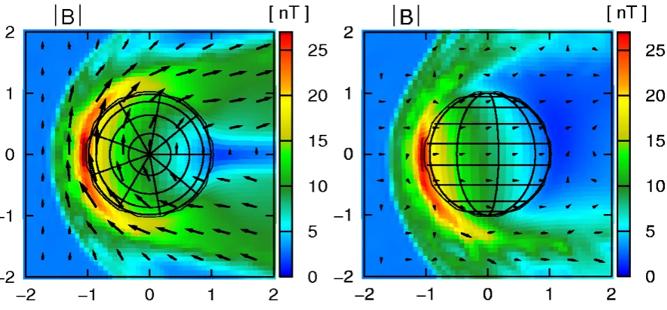
Fig. 4. Hybrid simulation: Distribution of the magnetic field strength in thexyplane (left) andxzplane (right).

hybrid simulations, there is a correlation between the proton velocity and electric field variations which is clearly indi-cated by Figs. 2, 3a. Maximal and minimal values of the os-cillating electric field and proton velocity are corresponding to each other. In spite of the fluctuations, the average veloc-ity in the hybrid simulations agrees with that of the MHD model. However, at the ICB, the proton’s velocity in the hy-brid model does not vanish. This might be related to a proton drift through the ICB which is caused by the nonzero electric field at the boundary. An additional possible reason is that a few energetic protons can cross the ICB.

A quite good agreement between the models appears for the magnetic field profiles along most of the mag-netosheath. The magnetic field behavior in the subsolar magnetosheath may be described as follows: the magnetic field increases monotonically from the bow shock towards the ICB. The scaling of the magnetic field maximum is

B∼√4πρswusw. The factor of the total magnetic field

en-hancement is of the order of the solar wind Alfv´en Mach numberBmax/Bsw∼MA. In the MHD simulation, the

mag-netic field increases by a factor of 12 for MA=10. In the

hybrid simulation the magnetic field maximum is a bit less because of magnetic diffusion into the ionosphere. The mag-netic pressure has a steep rise towards the obstacle; it in-creases by a factor of 2 on a length scale 0.1Rm=340 km.

The growth of the magnetic pressure is accompanied by a simultaneous drop in the plasma pressure. The maximum of the magnetic pressure is approximately equal to the solar wind dynamic pressure. The position of the magnetic field maximum in the simulations coincides with the total density pile-up boundary.

The subsolar magnetosheath profiles of the magnetic field and electron density shown in Fig. 2 are rather similar to those obtained from Phobos-2 measurements (see Fig. 1a) and also from bi-ion fluid simulations by Sauer and Dubinin (2000).

In the hybrid simulations, the proton temperature has large oscillations appearing just after the shock. However, the av-erage value seems to be rather close to that obtained from the Rankine-Hugoniot equations.

In the ideal MHD simulations, the magnetic field has a very sharp decrease from the ICB towards the planet. The strong decrease in the magnetic pressure is compensated by a corresponding increase in the plasma pressure. This struc-ture can be unstable with respect to an interchange instabil-ity, which leads to the penetration of magnetic tubes into the ionosphere. In the hybrid simulations, the magnetic field penetrates inside the ionosphere because of magnetic diffu-sion effects.

Figures 4 and 5 present the distributions of the magnetic field strength and proton density in the xy and xz planes which are obtained in the hybrid simulation. In thexyplane, the distributions of the magnetic field and plasma density are rather symmetrical, whereas in the xzplane one can see a strong asymmetry in the direction of the solar wind convec-tion electric field, related to finite gyro-radius effects. Such asymmetries were also reproduced in other hybrid simula-tions (e.g. Shimazu, 2001; Kallio and Janhunen, 2002).

The magnetosheath magnetic barrier is indicated in Fig. 4 by the red color in the dayside magnetosheath region. Its size along the y-direction is about 2RM. This is similar to

Fig. 5. Hybrid simulation: Distribution of the proton density in thexyplane (left) andxzplane (right).

solar wind magnetic field into the ionosphere because of the magnetic diffusion effects.

The distribution of the solar wind protons shown in Fig. 5 is rather patchy. At the subsolar bow shock, the proton den-sity is of the same order of magnitude as that in the MHD simulation. But in the middle part of the magnetosheath, the hybrid proton density is somewhat lower than that calculated in the MHD model. In the vicinity of the ICB, the proton density has a very sharp decrease similar to the MHD re-sult. There is a distinct slightly expanding boundary where the proton density drops to zero.

Figures 6, 7, 8 show the MHD model distributions of the magnetic field strength, proton density and plasma pressure in the magnetosheath in two planes, xy andxz, which are coplanar and perpendicular to the IMF, respectively. The undisturbed IMF lines are shown in thexy plane as straight lines along the y-direction. Contrary to the hybrid model, the distributions of the magnetic field and plasma parameters are symmetrical in both planes. The coordinates x, y are given in units of the planetary radius. In Fig. 6 one can see explic-itly the enhanced magnetic field strength in the magnetic bar-rier (red layer) adjacent to the dayside magnetopause. In the magnetosheath, the behavior of the plasma pressure is oppo-site to that of the magnetic field strength. The proton density has a systematic decrease from the bow shock towards the obstacle.

Good agreement between the MHD and hybrid magnetic field profiles in the magnetosheath of Mars can be interpreted on the basis of the following physical reasons: in the ideal MHD model, the physical reason for the magnetic pile-up is a stretching of the magnetic field lines which are frozen-in to the magnetosheath plasma flow. In the hybrid model, the

magnetic field is frozen-in only to electrons, but not to pro-tons, but effectively, it behaves as if it were frozen-in to the whole plasma in most of the dayside magnetosheath. This means that the relative speed of the electrons and protons (electric current speed) is much smaller than the bulk speed of the protons. To check this condition we express the elec-tron velocity using Eq. (19),

ue=up+

ni

n(ui −up)− c

4π ne∇ ×B. (22)

Eliminating the electron velocity from induction Eq. (21), we obtain

∂B

∂t = ∇ ×(up×B)+ ∇ ×

hn_i

n(ui−up)×B)

i −

∇ ×

₁

4π en(∇ ×B)×B

. (23)

With dimensionless quantities normalized to the solar wind parameters and a length scale for the magnetic barrier1m,

Eq. (23) yields

∂B˜

∂_t˜ = ∇ ×(u˜p× ˜B)+ ∇ × hn_i

n(u˜i − ˜up)× ˜B)

i −

δp

MA1m

∇ × ₁

˜

n(∇ × ˜B)× ˜B

, (24)

where δp is the inertial scale of the solar wind protons

δp=cpMp/

√

4π nswe. The second term can be neglected

while the ratio of the heavy ion density to the total density is small. It becomes important only in the vicinity of the ICB. The third term in Eq. (24) has a small coefficient

ξ = 1

MA

δp

1m

1.5

1.0

0.5

0.0

0.5

1.0

x

1.5

1.0

0.5

0.0

0.5

1.0

1.5

y

0.

5.

10.

15.

20.

25.

30.

B

nT

1.5

1.0

0.5

0.0

0.5

1.0

x

1.5

1.0

0.5

0.0

0.5

1.0

1.5

z

0.

5.

10.

15.

20.

25.

30.

B

nT

Fig. 6. MHD model: Distribution of the magnetic field strength in thexyplane (left) andxzplane (right).

For the input solar wind parameters (11) we findMA=10,

δp=114 km. Taking the scale 1m∼0.1RM from the

mag-netosheath profiles presented in the figures, we estimate the coefficientξ=0.034. Therefore, for most of the dayside mag-netosheath, we can neglect the last term in the induction Eq. (24). This means that the magnetic field can be con-sidered to be frozen-in to the plasma, as it is assumed in the ideal MHD. However, the last term becomes important in the vicinity of the ICB, where the magnetic field has a large gra-dient.

In the MHD simulation, the assumed ratio of specific heat (κ=5/3) is relevant to the solar wind protons and oxygen atomic ions. In the hybrid simulations, the protons and ions are treated kinetically, but electrons are considered to be a polytropic gas (pe∼nκe) with the polytropic indexκ=2

which is different from that used in the MHD calculations. However, this difference does not greatly affect the mag-netosheath profiles, because the electron pressure is rather small compared to the proton pressure.

As distinguished from other MHD codes, the present MHD code based on the frozen-in coordinates does not have a numerical magnetic diffusion. Therefore, it describes an ideal MHD flow with frozen-in magnetic field lines. In this model, the magnetosheath plasma flow produces a stretching of the magnetic field lines, which results in the formation of the magnetic barrier in front of the ICB where the protons are stopped. In the ideal one-fluid MHD model, the inter-planetary magnetic field is enhanced just before the proton stoppage boundary associated with the ICB, and the

mag-netic field lines cannot penetrate inside the cavity. In a two-fluid MHD and also in hybrid models, the magnetic field lines and protons are decoupled and thus the interplanetary magnetic field lines are allowed to penetrate through the pro-ton stoppage boundary. However, numerical diffusion effects usually lead to smoothing of the magnetic field boundaries. The present hybrid model has sufficient resolution to pro-duce a rather distinct boundary of the proton cavity which coincides with the magnetic field maximum at the subsolar region. However, the magnetic field variation through the cavity boundary is rather smooth.

6 On magnetic field diffusion into the ionosphere

In this section we discuss physical reasons for the magnetic field diffusion into the ionosphere which is seen in the hybrid simulations.

The cold, heavy ions inside the ionosphere are assumed to obey the equations

Mi

_∂u

i

∂t +ui∇ui

=e(E+1

cui×B)

−MiKDN0ui. (26)

1.5

1.0

0.5 0.0

0.5

1.0

x

1.5

1.0

0.5

0.0

0.5

1.0

1.5

y

0.

2.

4.

6.

8.

10.

12.

14.

n

cm

1.5

1.0

0.5

0.0

0.5

1.0

x

1.5

1.0

0.5

0.0

0.5

1.0

1.5

z

0.

2.

4.

6.

8.

10.

12.

14.

n

cm

Fig. 7. MHD model: Distribution of the proton density inxyplane (left) andxzplane (right).

1.5

1.0

0.5

0.0

0.5

1.0

x

1.5

1.0

0.5

0.0

0.5

1.0

1.5

y

0.

0.1

0.2

0.3

0.4

0.5

0.6

P

nPa

1.5

1.0

0.5 0.0

0.5

1.0

x

1.5

1.0

0.5

0.0

0.5

1.0

1.5

z

0.0

0.1

0.2

0.3

0.4

0.5

P

nPa

Fig. 8. MHD model: Distribution of the plasma pressure inxyplane (left) and inxzplane (right).

We introduce the normalized physical quantities, B= ˜BB∗, ui = ˜ui

cE∗

B∗ , t= ˜t

RMB∗

cE∗ ,

r = ˜rRM, E= ˜EE∗, (27)

and rewrite Eq. (26) in a dimensionless form

µ

_∂u˜

i

∂t + ˜ui∇ ˜ui

=η(E+ ˜ui× ˜B)− ˜ui, (28)

where

µ= cE

∗

RMKDN0B∗

, η= eB

∗

MicKDN0

. (29)

andηalong thexaxis for the normalization parameters

B∗=10 nT, E∗=0.1 V/km. (30)

These normalization parameters are of the order of the char-acteristic values of the magnetic and electric field as obtained in the hybrid simulation in the ionospheric region. One can see in Fig. 9 that coefficientµis rather small until the altitude of 270 km.

Neglecting the term proportional to the small coefficient

µ, we obtain the linear algebraic equation for the ion velocity

η(E˜ + ˜ui× ˜B)− ˜ui =0. (31)

Assuming the magnetic field along they direction, we find the ion velocity components as linear functions of the electric field components,

˜

ui,x =

η

1+η2_B˜2 ˜

Ex−

η2B˜

1+η2_B˜2 ˜

Ez,

˜

ui,y =ηE˜y,

˜

ui,z=

η

1+η2_B˜2 ˜

Ez+

η2B˜

1+η2_B˜2 ˜

Ex. (32)

Using Eq. (32) for the electric current of the ions ji=enV∗u˜i, one can obtain Ohm’s law for the ions with a

tensor conductivity,

ji =6E. (33)

The nondiagonal components of the conductivity tensor be-come of the order of the diagonal ones at altitudes exceeding 225 km. Below, the conductivity tensor can be considered as a diagonal6=σI, whereσis a scalar conductivity,

σ = nie 2

MiKDN0

. (34)

At the subsolar region, considering the electric field to be alongz, we have the equation

Ez =σjz. (35)

In the subsolar region, the length scale of the magnetic field variation along the x-direction is much smaller than the length scales along the y- and z-directions (see Fig. 4). Therefore, we assume the derivative along the x-axis to be much larger than those along the y- and z-directions. From Eq. (35) and the Maxwellian equations, we obtain the mag-netic diffusion equation

∂By

∂t = ∂ ∂x

νm

∂By

∂x

, (36)

whereνmis the magnetic diffusion coefficient,

νm=

c2

4π σ. (37)

0 50 100 150 200 250 300 350

1.105 1.104 1.103 0.01

0.1 1 10

(x-R )[km]

e

m( ), h( )

(x),

x

x

h( )

x

m( )

x

e

(x)

Fig. 9. Altitude dependence of the dimensionless parameters: dash,

dash-and-dot, and solid lines are corresponding toη,, andµ, re-spectively.

The time scale of the magnetic field diffusion is

τd =

1

c24π σ 1s, (38)

where1s is the subsolar altitude of the ICB. We introduce a

dimensionless parameterthat is a ratio of the diffusion time scale to the simulation timet∗∼2500 s,

(x)= 4π e 2₁2

sni

c2_t∗_k

DN0Mi

. (39)

Small values of this parameter mean that the simulation time exceeds the magnetic diffusion time, and thus the magnetic field can penetrate into the ionosphere until the Martian sur-face during the simulation run. Figure 9 shows the altitude dependence of the diffusion time parameter(x). This pa-rameter becomes less than 1 at the altitude≤285 km, where the magnetic field diffusion becomes important due to colli-sions with neutrals. Above this altitude, a magnetic diffusion might have only numerical reasons.

7 Conclusions

The solar wind interaction with Mars is considered on a ba-sis of the ideal MHD and hybrid models. The magnetosheath profiles of the magnetic field and plasma parameters, calcu-lated in both models, are compared.

the heavy ions dragged by the electric field from the iono-sphere in the hybrid simulation. Acceleration of these ions leads to a decrease in the average speed of the protons and a corresponding increase in the magnetosheath thickness.

However, good agreement between the models is found for the magnetic field and plasma parameters just after the bow shock. This means that in spite of the oscillations, the hybrid model can reproduce a thermalization of plasma at the bow shock and satisfy the Rankine-Hugoniot conditions based on conservation of mass, momentum and energy.

A particular good agreement between the MHD and hy-brid models is obtained for the subsolar magnetic field pro-files between the bow shock and the ICB. This allows us to suggest that the physical mechanism of the magnetosheath magnetic barrier described by the ideal MHD model is also valid for relatively small bodies like Mars. In the ideal MHD model, the physical reason for the magnetosheath magnetic barrier is a stretching of the magnetic field lines which are frozen-in to the plasma in the magnetosheath flow. In the hy-brid model, the magnetic field generally is frozen-in to the electrons, but not to the protons, but effectively, it behaves as if it were frozen-in to the whole plasma in the part of the day-side magnetosheath where the ionospheric ions are a minor component. This means that the relative speed of the elec-trons and protons (electric current speed) is much smaller than the bulk speed of the protons. This condition is not fulfilled in the vicinity of the ICB, where the electric cur-rent speed becomes comparable to the bulk velocity, and the magnetic field is frozen-in to the electrons only.

We have focused our analysis only on the magnetosheath region above the proton cavity, because the enhanced mag-netic field inside the cavity cannot be described by the ideal MHD model. The induced magnetosphere is reproduced by the hybrid model, but the magnetic field distribution and the MPB structure are greatly smoothed by the numerical diffu-sion. Therefore, the hybrid model does not predict a sudden jump in the magnetic field strength at the MPB, as it is iden-tified in the observations (Nagy et al., 2004).

The physical reasons for the magnetic field penetration into the ionosphere are analyzed. The magnetic field dif-fusion due to collisions with the neutral particles is found to be essential at the altitude of 55 km below the ICB. For the conditions of the hybrid simulations, the magnetic field pen-etrates from ICB until the diffusion zone because the elec-tron pressure itself is not sufficient to support the magnetic boundary.

Acknowledgements. This work was supported by grant Y 436RUS17/121/05 and Mo 539/13-2 from the “Deutsche Forschungsgemeinschaft”. Additional support is due to grant 04-05-64088 from the Russian Foundation of Basic Research, by Programs 2.17 and 16.3 of the Russian Academy of Sciences, by project P17100–N08 from the Austrian “Fonds zur F¨orderung der wissenschaftlichen Forschung”, and also by project I.2/04 from “ ¨Osterreichischer Austauschdienst”.

Topical Editor I. A. Daglis thanks two referees for their help in evaluating this paper.

References

Biernat, H. K., Erkaev, N. V., and Farrugia, C. J.: Aspects of MHD flow about Venus, J. Geophys. Res., 104, 12 617–12 626, 1999. Biernat, H. K., Erkaev, N. V., and Farrugia, C. J.: MHD effects

in the Venus magnetosheath including mass loading, Adv. Space Res., 28, 833–839, 2001.

Breus, T. K., Krymskii, A. M., Lundin, R., Dubinin, E. M., Luh-mann, J. G., Yeroshenko, Y. G., Barabash, S. V., Mitnitskii, V. Y., Pissarenko, N. F., and Styashkin, V. A.: The solar wind interac-tion with Mars: considerainterac-tion of Phobos-2 mission observainterac-tions of an ion composition boundary on the dayside, J. Geophys. Res., 96, 11 165–11 174, 1991.

Brecht, S. H., Ferrante, J. R., and Luhmann, J. G.: Three-dimensional simulations of the solar wind interaction with Mars, J. Geophys. Res., 98, 1345–1357, 1993.

Brecht, S. H.: Hybrid simulations of the magnetic topology of Mars, J. Geophys. Res., 102, 4743-4750, 1997.

B¨oßwetter, A, Bagdonat, T., Motschmann, U., and Sauer, K.: Plasma boundaries at Mars: a 3-D simulation study, Ann. Geo-phys., 22, 4363–4379, 2004,

http://www.ann-geophys.net/22/4363/2004/.

Chamberlain, J. W. and Hunten, D. M.: Theory of planetary atmo-spheres, Academic Press, New York, 1987.

Chen, R. H., Cravens, T. E., and Nagy, A. F.: The Martian iono-sphere in light of the Viking observations, J. Geophys. Res., 83, 3871–3876, 1978.

Erkaev, N. V., Farrugia, C. J., and Biernat, H. K.: Effects on the Jovian magnetosheath arising from solar wind flow around non-axial bodies, J. Geophys. Res., 101, 10 665–10 672, 1996. Erkaev, N. V., Farrugia, C. J., and Biernat, H. K.: Comparison of

gasdynamics and MHD predictions for magnetosheath flow, in: NATO ASI Series, Polar Cap Boundary Phenomena, edited by: Moen, J., Egeland, A., and Lockwood, M., Kluwer Academic Publisher, Dordrecht, The Netherlands, 509, p. 27–40, 1998. Erkaev, N. V., Farrugia, C. J., and Biernat, H. K.:

Three-dimensional, one-fluid, ideal MHD model of magnetosheath flow with anisotropic pressure, J. Geophys. Res., 104, 6877–6888, 1999.

Erkaev, N. V., Farrugia, C. J., and Biernat, H. K.: The role of the magnetic barrier in the Solar wind-magnetosphere interaction, Planet. Space Sci., 51, 745–755, 2003.

Hanson, W. B. and Mantas, G. P.: Viking electron temperature mea-surements: Evidence for a magnetic field in the Martian iono-sphere, J. Geophys. Res., 93, 7538–7544, 1988.

Israelevich, P. L., Gombosi, T. I., Ershkovich, A. I., DeZeeuw, D. L., Neubauer, F. M., and Powell, K. G.: The induced mag-netosphere of comet Halley, 4, Comparison of in situ observa-tions and numerical simulaobserva-tions, J. Geophys. Res., 104, 28 309– 28 319, 1999.

Kallio, E. and Luhmann, J. G.: Charge exchange near Mars: The solar wind absorption and energetic neutral atom production, J. Geophys. Res., 102, 22 183–22 197, 1997.

Kallio, E. and Janhunen, P.: Ion escape in a quasi-neutral hybrid model, J. Geophys. Res., 107, 1035, doi:10.1029/2001J000090, 2002.

Kotova, G., Verigin, M., Remizov, A., Rosenbauer, H., Livi, S., Szeg¨o, K., Tatrallyay, M., Slavin, J., Lemaire, J., Schwingen-schuh, K., and Zhang, T. L.: Study of the solar wind deceleration upstream of the Martian terminator bow shock, J. Geophys. Res., 102, 2165–2173, 1997.

Liu, Y., Nagy, A. F., Gombosi, T. I., DeZeeuw, D. L., and Powell, K. G.: The solar wind interaction with Mars: results of three-dimensional threespecies MHD studies, Adv. Space Res., 27, 1837–1846, 2001.

Ma, Y., Nagy, A. F., Sokolov, I. V., and Hansen, K. C.: Three-dimensional, multispecies, high spatial resolution MHD studies of the solar wind interaction with Mars, J. Geophys. Res., 109, A07211, doi:10.1029/2003JA010367, 2004.

Nagy, A. F., Winterhalter, D., Sauer, K., Cravens, T. E., Brecht, S., Mazelle, C., Crider, D., Kallio, E., Zakharov, A., Dubinin, E., Ve-rigin, M., Kotova, G., Axford, W. I., Bertucci, C., and Trotignon, J. G.: The plasma environment of Mars, Space Sci. Rev., 111, 33–114, 2004.

Petrinec, S. M. and Russell, C. T.: Hydrodynamic and MHD equa-tions across the bow shock and along the surfaces of planetary obstacles, Space Sci. Rev., 79, 757–791, 1997.

Pudovkin, M. I. and Semenov, V. S.: Stationary frozen–in coordi-nate system, Ann. Geophys., 33, 429–433, 1977,

http://www.ann-geophys.net/33/429/1977/.

Riedler, W., Schwingenschuh, K., Lichtenegger, H., M¨ohlmann, D., Rustenbach, J., Weroshenko, Y., Achache, J., Slavin, J., Luh-mann, J. G., and Russell, C. T.: Interaction of the solar wind with the planet Mars: Phobos- 2 magnetic field observations, Planet. Space Sci., 39, 75–81, 1991.

Rosenbauer, H., Shutte, N., Apathy, I., Galeev, A., Gringauz, K., Gr¨unwaldt, H., Hemmerich, P., Jockers, K., Kiraly, P., Kotova, G., Livi, S., Marsch, E., Richter, A., Riedler, W., Remizov, T., Schwenn, R., Schwingenschuh, K., Steller, M., Szeg¨o, K., Veri-gin, M., and Witte, M.: Ions of Martian origin and plasma sheet in the Martian magnetoshere/initial results of the TAUS experi-ment, Nature, 341, 612–614, 1989.

Sauer, K., Roatsch, Th., Motschmann, U., M¨ohlmann, D., Schwin-genschuh K., and Riedler, W.: Plasma boundaries at Mars dis-covered by the Phobos 2 magnetometers, Ann. Geophys., 8, 661– 670, 1990,

http://www.ann-geophys.net/8/661/1990/.

Sauer, K., Bogdanov, A., and Baumgaertel, K.: Evidence of an ion composition boundary (protonopause) in bi-ion fluid simulations of solar wind mass loading, Geophys. Res. Lett., 21, 2255–2258, 1994.

Sauer, K. and Dubinin, E.: The nature of the Martian .obstacle boundary., Adv. Space Res., 26, 1633–1637, 2000.

Shimazu, H.: Three-dimensional hybrid simulation of solar wind interaction with unmagnetized planets, J. Geophys. Res., 106, 8333–8342, 2001.

Spreiter, J. R. and Stahara, S. S.: A new predictive model for de-termining solar wind – terrestrial planet interactions, J. Geophys. Res., 85, 6769–6777, 1980.

Zwan, B. J. and Wolf, R. A.: Depletion of solar wind plasma near a planetary boundary, J. Geophys. Res., 81, 1636–1648, 1976. Vignes, D., Mazelle, C., Rme, H., Acuna, M. H., Connerney, J. E.