DBSCAN: Optimal Rates For Density-Based Cluster
Estimation
Daren Wang [email protected]
Department of Statistics University of Chicago Chicago, IL 60637, USA
Xinyang Lu [email protected]
Mathematical Sciences Department Lakehead University
Thunder Bay, ON P7B 5E1, Canada
Alessandro Rinaldo [email protected]
Department of Statistics and Data Science Carnegie Mellon University
Pittsburgh, PA 15213, USA
Editor:Ingo Steinwart
Abstract
We study the problem of optimal estimation of the density cluster tree under vari-ous smoothness assumptions on the underlying density. Inspired by the seminal work of Chaudhuri et al. (2014), we formulate a new notion of clustering consistency which is bet-ter suited to smooth densities, and derive minimax rates for clusbet-ter tree estimation under H¨older smooth densities of arbitrary degree. We present a computationally efficient, rate optimal cluster tree estimator based on simple extensions of the popular DBSCAN algo-rithm of Ester et al. (1996). Our procedure relies on kernel density estimators and returns a sequence of nested random geometric graphs whose connected components form a hierarchy of clusters. The resulting optimal rates for cluster tree estimation depend on the degree of smoothness of the underlying density and, interestingly, match the minimax rates for den-sity estimation under the sup-norm loss. Our results complement and extend the analysis of the DBSCAN algorithm in Sriperumbudur and Steinwart (2012). Finally, we consider level set estimation and cluster consistency for densities with jump discontinuities. We demonstrate that the DBSCAN algorithm attains the minimax rate in terms of the jump size and sample size in this setting as well.
Keywords: DBSCAN; density-based clustering; cluster tree; minimax optimality; H¨older smooth density.
1. Introduction
Clustering is one of the most basic and fundamental tasks in statistics and machine learning, used ubiquitously and extensively in the exploration and analysis of data. The literature on this topic is vast, and practitioners have at their disposal a multitude of algorithms and heuristics to perform clustering on data of virtually all types. However, despite its
c
importance and popularity, rigorous statistical theories for clustering, leading to inferen-tial procedures with provable theoretical guarantees, have been traditionally lacking in the literature. As a result, the practice of clustering, a central tasks in the analysis and ma-nipulation of data, still relies in many cases on methods and heuristics of unknown or even dubious scientific validity. One of the most striking instances of such a disconnect is the DBSCAN algorithm of Ester et al. (1996), an extremely popular and relatively efficient (see Gan and Tao, 2015; Wang et al., 2015) clustering methodology whose statistical properties have been properly analyzed only very recently: see Sriperumbudur and Steinwart (2012), Jiang (2017a) and Steinwart et al. (2017).
In this paper, we provide a complementary and thorough study of DBSCAN, and show that this simple algorithm can deliver optimal statistical performance indensity-based clus-tering. Density-based clustering (see, e.g., Hartigan, 1981) provides a general and rigorous probabilistic framework in which the clustering task is well-defined and amenable to statis-tical analysis. Given a probability distribution P on Rd with a corresponding continuous
density pand a fixed thresholdλ≥0, the λ-clustersof p are the connected components of the upper λ-level set of p, the set {x ∈ Rd:p(x) ≥ λ} of all points whose density values
exceed the levelλ. With this definition, clusters are the high-density regions, subsets of the support ofP with the largest probability content among all sets of the same volume.
As noted in Hartigan (1981), the hierarchy of inclusions of all clusters of p is a tree structure indexed byλ >0, called thecluster tree ofp. The chief goal of density clustering is to estimate the cluster tree of p, given an i.i.d. sequence{Xi}ni=1 of points with common
distributionP. A cluster tree estimator is also a tree structure, consisting of a hierarchy of nested subsets of the sample points, and typically relies on non-parametric estimators of p in order to determine which sample points belong to high-density regions ofp. A cluster tree estimator is deemed accurate if, with high probability, the hierarchy of clusters it encodes is close to the hierarchy that would have been obtained shouldp be known.
Density-based clustering, an instance of hierarchical clustering, enjoys several advan-tages: (1) it imposes virtually no restrictions on the shape, size and number of clusters, at any level of the tree; (2) unlike flat (i.e. non-hierarchical) clustering, it does not require a pre-specified number of clusters as an input and in fact the number of clusters itself is a quantity that may change depending on the level of the tree; (3) it provides a multi-resolution representation of all the clustering features of p across all levels λat the same time; (4) it allows for an efficient representation and storage of the entire tree of clusters with a compact data structure that can be easily accessed and queried, and (5) the main object of interest for inference, namely the cluster tree of p, is a well-defined quantity.
because of this generality, these consistency rates do not directly reflect any degree of reg-ularity or smoothness of the underlying density. In particular, it remains unclear whether cluster tree estimation would be easier with smoother densities.
In this paper we provide further contributions to the theory of density based clustering by deriving novel, nearly minimax-optimal rates for cluster tree estimation that depend explicitly on the smoothness of the underlying density function. Our results further confirm that the smoother the density the faster the rate of consistency for the cluster tree estimation problem, a finding that is consistent with analogous results about non-parametric density estimation. Interestingly, our rates match those for estimating smooth densities in the L∞ norm. To the best of our knowledge, this finding and the implication that density based clustering is no easier – at least in our setting – than density estimation, has not been rigorously shown before. In order to account explicitly for the smoothness of the density, we have developed a new criterion for cluster consistency that is better suited for smooth densities. In terms of procedures, we consider cluster tree estimators that arise from applying a very simple generalization of the well-known DBSCAN algorithm and are computationally efficient. Furthermore, our DBSCAN-based estimator is minimax optimal over arbitrary smooth densities according to our notion of consistency under appropriate conditions.
Related work
compu-tational complexity while Jiang et al. (2019) studied DBSCAN under possibly adversarial contamination of the input data.
In a parallel and important line of work, Steinwart (2011, 2015) developed a rigorous, measure-theoretic approach to density-based clustering whereby the cluster tree is recovered by estimating the lowest split level of the density and then proceeding recursively. The cor-responding results demonstrate a direct link between density based clustering and optimal level set estimation. This approach was applied in Sriperumbudur and Steinwart (2012) to show that the DBSCAN algorithm yield consistent estimator of density trees, a result that was then extended in Steinwart et al. (2017) to allow for more general, KDE-based procedures. Our work built directly upon the contributions of Chaudhuri et al. (2014) and Steinwart (2015).
Organization of the paper
The rest of the paper is organized as follows. In Section 3, we describe the DBSCAN algo-rithm and establish its connections with non-parametric density estimation. In Section 4 we introduce a new notion of cluster consistency, called δ-consistency that is tailored to H¨older-continuous densities. We describe a DBSCAN-based algorithm for clustered tree estimation that is computational efficient and delivers nearly optimal minimax rates that depend explicitly on the degree of smoothness of the underlying density, whereby cluster tree of smoother densities can be estimated at faster rates. Interestingly and, perhaps surprisingly, for the class of DBSCAN-based algorithms we consider, we observe a trade-off between statistical optimality and computational cost for smoother H¨older densities of degree α >1. In these situations, minimax rates can still be achieved by our computation-ally efficient algorithm provided that the underlying density satisfies additional geometric regularity conditions around the split levels. Such conditions are relatively mild and have been exploited before; see in particular Steinwart (2015). Finally, in Section 5 we consider a different scenario in which the underlying density exhibits jump discontinuities. We are particularly interested in level set and cluster estimation at the jump, with the assumption that the size of the discontinuity is vanishing when n→ ∞so that clustering becomes in-creasingly difficult. We show that, with suitable inputs, the DBSCAN algorithm returns a Devroye-Wise type of estimator which is minimax optimal for cluster recovery and level set estimation. In addition, we derive the minimax scaling for the size of the jump discontinuity.
Notation
We denote with p a density for the distribution P of the i.i.d. sample {Xi}ni=1 ⊂ Rd. For
a constant λ >0, we set L(λ) = {p ≥λ} to be the λ-upper upper level set of the density p. We use Tp to denote the cluster tree generated by the density p and Tb to density any estimator ofTp. We use subscriptnto emphasize any global variable which may change with
respect ton. Lrepresents the Lebesgue measure inRdandB(x, r) the closedddimensional
Euclidean ball centered at x with radius r and Vd = L(B(0,1)) the volume of the unit
set A⊂Rd we set
Ah=
[
x∈A
B(x, h) and A−h={x∈A:B(x, h)⊂A}. (1)
For any two real sequences{an}∞n=1 and{bn}∞n=1 we writean=O(bn) if there existsC >0
such that lim supn→∞|an/bn|< Cand writean= Θ(bn) ifan=O(bn) andbn=O(an). For
any two closed subsets A and B of Rn, we use d(A, B) = infx∈A,y∈Bkx−yk to represent
the ordinary distance between them.
2. Cluster Trees Estimation
LetP be a probability distribution with a continuous1 Lebesgue densitypand with support Ω⊂Rd. For anyλ≥0, let{x∈Ω :p(x)≥λ}be theλ-upper level set ofpand theλ-cluster
ofpare the connected components ofL(λ). See Appendix A for definition of connectedness. Notice that the set of all clusters is an indexed collection of subsets of Ω, whereby each cluster of p is assigned the index λ associated to the corresponding super-level set L(λ), and that many clusters may be indexed by the same level λ. The cluster tree of p is the collection Tp of all clusters ofp, that is
Tp ={L(λ)}λ≥0.
We can think of the cluster tree of p as the function defined on [0,∞) and for eachλ≥0, it returns the set of λ-clusters of p. Thus, Tp(λ) consists of disjoint connected subsets of
Ω. We remark that, since the densitypis unique only up to sets of Lebesgue measure zero, the cluster tree Tp is also not unique. In fact, Steinwart (2015) shows that there exists a
well-defined notion of cluster tree for the distribution P that is independent of the choice of the density. Furthermore, if P admits an upper semi-continuous density p, then the cluster tree is in fact composed of the hierarchy of the (closures of the) upper level sets of such density. As P is assumed, throughout most of the article, to have a density that is continuous everywhere on its support, when we speak of “the” density of P, we will refer to this canonical choice.
The concept of cluster tree owes its name to the easily verifiable property (see Hartigan (1981)) that if A and B are elements of Tp, i.e. distinct clusters of p, then A∩B =∅ or
A⊆B orB ⊆A. This induces a partial order on the set of clusters. In particular, for any λ1≥λ2 ≥0, ifA∈Tp(λ1) andB∈Tp(λ2) then eitherA∩B =∅ orB ⊆A. As a result,Tp
can be represented as a dendrogram with height indexed by λ≥0. We refer to Kim et al. (2016) for a formal definition of the dendrogram encoding a cluster tree.
Let {Xi}ni=1 be i.i.d. samples fromP. In order to estimate the cluster tree of pwe will
consider tree-valued estimators, defined below.
Definition 1. A cluster tree estimator ofTp is a collectionTbnof subsets of{Xi}ni=1 indexed
by [0,∞) such that
•for eachλ≥0,Tbn(λ)consists of disjoint subsets of{Xi}ni=1 (including, possibly the empty
set), called clusters, and
• Tbn satisfies the tree property: for any λ1 ≥ λ2 ≥0, if A ∈Tbn(λ1) and B ∈ Tbn(λ2) then either A∩B =∅ or A⊆B.
It is important to realize that, while the cluster treeTpis a collection of connected subsets
of the support of p, the cluster tree estimators considered in this paper are collections of subsets of the sample points.
In order to quantify how well a cluster-tree estimator approximates the true cluster tree, we will make use of the notion of cluster tree consistency put forward by Chaudhuri et al. (2014).
In detail, let An denote a collection of connected subsets of the support of p, which may depend on n. A cluster tree estimator Tbn is consistent with respect to An if, with probability tending to 1 as n → ∞, the following holds simultaneously over all A and A0 in An: the smallest clusters in Tbn containing A∩ {Xi}ni=1 and A0 ∩ {Xi}ni=1 are disjoint. The requirement for consistency outlined above is rather natural: if a cluster tree is deemed consistent with respect to the sequence An, then it should, with probability tending to 1,
cluster the sample points perfectly well, as if we had the ability of verifying, for each pair of sample pointsXi and Xj and each connected set A∈ An, whether bothXi and Xj are
inA.
We allowAn to grow larger and more complex withn, so that the cluster tree estimator
will be able to discriminate among clusters of p that are barely distinguishable given the size of the sample. An example of a sequence {An}∞n=1 is the set ofδn-separated clusters
according to Definition 2, where the parameter δn is taken to be vanishing asn→ ∞. The
sequence of target subsets {An}∞
n=1 may not be chosen to be too large: for example if An
equals to the set of all clusters of p, then, depending on the complexity of p, no cluster tree estimator need to be consistent. A natural way to define {An}∞n=1 is by specifying a separation criterion for sets, which may become less strict as n grows, and then populate each An using only the connected subsets of the support of pfulfilling such a criterion. In
particular, Chaudhuri et al. (2014) develop a criterion known as the (, σ)-separation, which requires two connected subsets A and A0 to be far apart from each other in terms of their “horizontal” distance d(A, B) and their “vertical” distance, in the sense that the smallest cluster containing both A and B should belong to a level set ofp indexed by a value of λ significantly smaller to the values indexing the level sets ofAandB. See Definition 10 below for details. One of the main contributions of this paper is to replace this rather general notion of separation by a simpler one, the δ-separation criterion in Definition 2, which is better suited deal with smooth densities. This allows us to derive new rates of consistency that depend explicitly on the smoothness of the density.
3. The DBSCAN Algorithm
The DBSCAN algorithm, first introduced in Ester et al. (1996), is an extremely popular methodology for “flat” clustering. In this section we introduce a simple generalization of DBSCAN, shown below in Algorithm 1, that yields cluster tree estimators and establish its connections with kernel density estimation.
Algorithm 1 The DBSCAN algorithm.
INPUT: i.i.d sample{Xi}ni=1, and h >0.
1. For each k∈ N, construct a graph Gh,k with nodes {Xi :|B(Xi, h)∩ {Xj}nj=1| ≥ k}
and edges (Xi, Xj) if kXi−Xjk<2h.
2. Compute C(h, k), the graphical connected components of Gh,k.
OUTPUT: {C(h, k), k∈N}.
For a fixed value ofk, Algorithm 1 is in fact a simplified version of the original DBSCAN procedure of Ester et al. (1996), where the parameters h and k are called instead Eps and MinPts, respectively. Notice that, unlike in the original formulation of DBSCAN, we do not distinguish between core and border points and, furthermore, we evaluate connectivity among the sample points using balls of radius 2h instead ofh. Such modifications have no impact on the rates of consistency we obtain but simplify the derivations.
Assuming h > 0 fixed, by sweeping through all the possible values of k, Algorithm 1 produces a sequence of nested geometric graphsTbn={C(h, k)}k∈N. It is immediate to see that Tbn forms a cluster tree estimator over the sample points {Xi}ni=1; see Definition 1. This is because, for each k1 ≤k2,
[
{Xi:|B(Xi,h)∩{Xj}nj=1|≥k2}
B(Xi, h)⊆
[
{Xi:|B(Xi,h)∩{Xj}nj=1|≥k1}
B(Xi, h).
In practice, Algorithm 1 can be efficiently implemented using a union-find structure in such a way that the set C(h, k) of the maximal connected components of Gh,k can be
computed without using the potentially expensive breadth-first search or depth-first search algorithms. The resulting cluster tree algorithm is simpler than the estimator based on Wishart’s algorithm proposed in Chaudhuri et al. (2014). Indeed, the DBSCAN-based estimator is obtained from a sequence of node-induced sub-graphs of the 2h-neighborhood graph over the sample points. In contrast, Wishart’s algorithm entails taking node and edge-induced sub-graphs of the k-nearest neighborhood graph over {X1, . . . , Xn}, which
has higher computational complexity.
As explained in Sriperumbudur and Steinwart (2012), DBSCAN is implicitly using a kernel density estimator with kernel corresponding to the indicator function of the unit d-dimensional Euclidean ball to cluster the points. In detail, consider the density estimator
b
ph given by
x∈Rd7→
b ph(x) =
|B(x, h)∩ {Xi}ni=1|
nhdV d
= 1
nhdV d
n
X
i=1
K
x−Xi
h
, (2)
where
K(x) =
1 ifx∈Bd(0,1),
It is easy to see that pbh is a Lebesgue density, i.e. pbh(x) is a measurable, non-negative function and R
Rdpbh(x)dx= 1. Furthermore, E[pbh(x)] =ph(x) for all x∈R
d,where
ph(x) =
1 hdV
d
Z
Rd K
x−z
h
p(z)dz = P(B(x, h)) hdV
d
. (4)
For anyλ≥0, setDb(λ) ={x:pbh(x)≥λ} ∩ {Xi}ni=1 and b
L(λ) = [
Xj∈Db(λ)
B(Xj, h). (5)
Then, setting, for k >0, λk = nhkdV
d, one can see that, for clustering purpose, C(h, k) and
b
L(λk) convey the same information. Indeed from the definition ofLb(λk), it is straightforward to see that
Lemma 1. Two data points Xi and Xj are in the same connected component of the d
-dimensional set Lb(λk) if and only if they are in the same connected component of the graph
C(h, k).
The union of balls Lb(λ) is a renown estimator in the literature on level set estima-tion, originally studied in Devroye and Wise (1980) (see also Cuevas and Rodr´ıguez-Casal (2004)). In particular, with a suitable choice of the bandwidth parameter h and as n grows unbounded,Lb(λ) is a rate-optimal estimator of the level set L(λ) under various loss functions and appropriate assumptions on the underlying density.
4. Clustering Consistency for H¨older Continuous Densities
In this section we show that the DBSCAN algorithm 1 is consistent under H¨older smooth densities. Towards that end, we introduce a new notion of cluster tree consistency, called δ-consistency (see Section 4.2 below), which is well-suited to study cluster trees generated by smooth densities. We will show that DBSCAN, with suitable inputs, will return cluster tree estimators that nearly attain the corresponding minimax optimal rates and that those rates depend on the degree of smoothness of the density.
4.1. H¨older smooth densities
Below we give a recap of well-known results on non-parametric density estimation. Given vectors s = (s1, . . . , sd) in Nd and x = (x1, . . . , xd) in Rd, set |s| = s1 +· · ·+sd and
xs =xs1
1 . . . x
sd
d , and let
Ds= ∂
s1+···+sd
∂xs11 . . . ∂xsd
d
denote the differential operator. A function p:Rd → Ris said to belong the H¨older class
Σ(L, α) with parameters α >0 andL >0 if pis bαc-times continuously differentiable and, for all x, y∈Rd and alls∈
Ndwith |s|=bαc,
Notice that, when 0< α≤1, the H¨older condition reduces to the Lipschitz condition
|p(x)−p(y)| ≤Lkx−ykα, ∀x, y∈Rd.
Let pbh denote a kernel density estimator with bandwidthh and kernelK, that is
b ph(x) =
1 nhd n X i=1 K
x−Xi
h
.
Then, we obtain the standard bias-variance decomposition for the KDEs, namely
kpbh−pk∞≤ kpbh−phk∞+kph−pk∞.
In order to control the stochastic componentkpbh−phk∞we will invoke well-known concen-tration bounds from density estimation to conclude that, under appropriate and very mild assumptions onK, there exists a constantC1 >0, depending onkpk∞,dandK, such that,
for any γ >0 and alln large enough and assumingnhd≥1,
P(kpbh−phk∞≤an)≥1−e
−γ, (6)
where
an=C1
r
(γ+ log(1/h))
nhd . (7)
The verification of this bound can be found in many places in the literature; see, e.g., Gin´e and Guillou (2002), Sriperumbudur and Steinwart (2012), Jiang (2017b) and Kim et al. (2019). See Appendix B for details. As for the bias term kph−pk∞, if K is chosen to be a
α-valid kernel2 (see, e.g., Rigollet and Vert (2009)), then standard calculations yield that
kph−pk∞≤C2hα, (8)
for an appropriate constantC2 >0 depending onL andα. In particular, since this type of
kernels are polynomials supported on [0,1]d, they automatically satisfy the VC condition (see lemma 22 of Nolan and Pollard, 1987, for a justification).
Thus combining the bias in (6) and the variance in (8), we conclude that, with probability at least 1−e−γ, withγ any positive number,
kpbh−pk∞≤C1
r
γ+ log(1/h) nhd +C2h
α. (9)
Setting, e.g.,γ = logn, the optimal choice of the bandwidth is
h
logn
n
2α+d
, (10)
leading to the final rate of
logn n
2αα+d
, which is in fact minimax optimal.
2. For a fixedα > 0, a functionK:Rd→Ris an α-valid kernel ifRRdK(x)dx= 1, has finiteLpnorm
for all p ≥ 1, R
Rdkxk
α
K(x)dx < ∞ and R
Rdx
s
K(x)dx = 0 for all s = (s1, . . . , sd) ∈ Zd such that
1≤Pd
i=1si ≤ bαc, where forx= (x1, . . . , xd) ∈R
d
,xs =Qd i=1x
si
i . See Definition 1 in Rigollet and
4.2. The δ-Separation Criterion
We now formulate a notion of cluster separation that is naturally suited to smooth densities and, for continuous densities is equivalent to separation in the merge distance of Eldridge et al. (2015) (see also Kim et al., 2016).
Definition 2. LetAandA0be subsets the support of the densitypand setλ:= infx∈A∪A0p(x).
Forδ ∈(0, λ), Aand A0 are said to be δ-separated if they belong to distinct connected com-ponents of the level set {x:p(x)> λ−δ}.
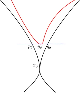
Unlike the separation criterion of Chaudhuri et al. (2014), which requires the specifica-tion of two parameters quantifying the horizontal and vertical displacement between clus-ters, δ-separation only uses one parameter The intuition behind the notion of δ-separation is simple: due to the smoothness of the density, the degrees of “vertical” and “horizontal” separation between clusters are coupled. This is illustrated in Figure 1 and best explained for the case of a density in Σ(L, α) with α ≤ 1. If A and A0 are δ-separated, then their distance is at least Lδ1/α
. As a result, the degree of separation between clusters of smooth densities can be described using only one parameter, a feature that we will exploit to derive new notion of consistency for clustering.
Definition 3. Let δ >0 and γ ∈(0,1). A cluster tree estimator based on an i.i.d. sample {Xi}ni=1 is(δ, γ)-accurate if, with probability no smaller than1−γ, for any pair of connected subsets AandA0 of the support that areδ-separated, exactly one of the following conditions holds:
1. at least one of A∩ {Xi}ni=1 andA0∩ {Xi}ni=1 is empty;
2. the smallest clusters in the cluster tree estimator containing A∩ {Xi}ni=1 and A0 ∩ {Xi}ni=1 are disjoint.
Let {δn}n be a vanishing sequence of positive numbers and a {γn} a vanishing sequence
in (0,1). We say that the sequence of cluster tree estimators {Tn}n, where Tn is based
on an i.i.d. sample {Xi}ni=1, is δ-consistent with rate δn if, for all n large enough, Tn is
(δn, γn)-accurate whereγn decays polynomially in n.
It is important to realize that the notion of δ-consistency is auniformnotion of consis-tency that is required to hold simultaneously over all possibly pairs ofδ-separated connected subsets of the support.
Theδ-separation criterion is closely related to the concept of themerge heightintroduced by Eldridge et al. (2015). In the context of hierarchical clustering, the merge height is used to describe the “height” at which two points or two clusters merge into one cluster; see Definition 9. In particular we show below in Lemma 4 that if two subsets Aand A0 of the support are δ-separated and infx∈A∪A0p(x) = λ, then their merge height is no larger than
λ−δ. To further emphasize how similar the two approaches are, we mention that our results about cluster consistency still hold for a slightly stronger notion of cluster consistency, whereby condition 2 in Definition 3 is replaced by the condition
2. there exists a levelλ∈[infx∈A∪A0f(x)−δ,infx∈A∪A0f(x)) such that A∩ {Xi}ni=1 and
The key difference betweenδ-consistency and this stronger version ofδ-consistency is that in the latter case we further constrain the split level forAandA0 in the cluster tree estimator to occur at a value less than infx∈A∪A0f(x) by an amount no larger thanδn. This is precisely
what is required for merge distance consistency; see Eldridge et al. (2015). We provide more detailed comparison in Section 6, where we further elucidate the differences between our notion of δ-separation and the (, σ)-separation criterion of Chaudhuri et al. (2014).
Figure 1: The left figure depicts a split level (defined in λ∗ Section 4.3) of the density p. The right figure depicts two setsAand A0 beingδ separated with respect toλ∗.
4.3. The split levels
One of the most impoertant features of a cluster tree is the collections of levels λat which the clusters split into two or more disjoint sub-clusters, which we refer to as split levels.
Such levels belong to the well-known class of “critical levels” in differential topology, which identify critical changes in the topology of the upper level sets ofp. See, for example, Hirsch (2012) for more details. In particular, the estimation of split levels is a central theme in the contributions of Sriperumbudur and Steinwart (2012) and in Steinwart (2015). Below, we provide a slightly different characterization of the split levels of continuous densities and relate it to the criterion of δ-separation of clusters. The notion of split levels will be important below in Section 4.4.2 in formalizing conditions under which computationally efficient and statistically optimal cluster tree estimation is feasible for H¨older densities with smoothness degree α > 1. It will also be used to demonstrate that we can easily remove false clusters from the cluster tree estimations returned by our algorithms (see Section 4.6).
Definition 4. Let p : Rd → R be a continuous density function. For a fixed λ∗ > 0, let {Ck}K
k=1 be the connected components of {p ≥λ
∗}. The value λ∗ is said to be a split level
of p if there exists a Ck such that Ck∩ {p > λ∗} has two or more connected components.
Proposition 1. Suppose that p : Rd → R is compactly supported and that A and A0 are subsets of two distinct connected components of {p ≥ λ1}. If A and A0 belongs to the same connected components of {p≥λ2}, where λ2 < λ1, then there is a unique split level
λ∗ ∈ [λ2, λ1) such that A and A0 belong to one connected component of {p ≥ λ∗} and to distinct connected components of {p > λ∗}.
Proposition 1 suggests that if two connected components merge into one as the density levelλdecreases, then there exists one and only one split level at which the corresponding merge takes place. Therefore, the following definition, which characterizes the split level of any two distinct clusters in a cluster tree, seems natural.
Definition 5. Suppose A and A0 are two open subsets of the support of p. Then A and A0
are said to split at level λ∗ ifA and A0 belong to one connected component of{p≥λ∗} and to two distinct connected components of {p > λ∗}.
In our next result we illustrate a direct link between the notion of split levels and the criterion of δ-separation introduced above. We will exploit this fact later in Section 4.6 to demonstrate how to prune the cluster tree estimators to yield accurate estimates of the split levels without producing false clusters.
Corollary 1. Let AandA0 be δ-separated. Then there exists a split levelλ∗ of the density, with
λ∗≤ inf
x∈A∪A0f(x)−δ,
such that A and A0 belong to one connected component of {p ≥ λ∗} and to two distinct connected components of{p > λ∗}.
4.4. Rate of consistency for the DBSCAN algorithm
We are now ready to present the main results of the paper, and derive rates of consistency for DBSCAN-based cluster tree estimators with respect to the criterion ofδ-separation and for H¨older smooth densities. Specifically, we will show that these estimators areδ-consistent with rate
δn≥C
log(n)
n
α
2α+d
, (11)
for an appropriate constantCthat depends onkpk∞,L,K andα. The above rates depend on the smoothness of the underlying density, with smoother densities leading to faster rates, and, as shown in Section 4.5, are in fact minimax optimal. This is one of the main contributions of this article and delivers an extension of the cluster consistency results of Chaudhuri et al. (2014), which are agnostic to the smoothness ofp.
4.4.1. Consistency for α≤1
(2010), Sriperumbudur and Steinwart (2012), Jiang (2017a) and Steinwart et al. (2017). We provide the details for completeness.
In order to demonstrate that DBSCAN isδ-consistent, it will be sufficient to show that the procedure provides an approximation to the upper level sets of pbh. This is done in
the next result, which relies on general, well-known, finite sample concentration bounds for KDEs along with standard calculations for the bias of a KDE; see Lemma 6 and Proposi-tion 7 in Appendix B.
Lemma 2. Assume that p ∈ Σ(L, α), where α ∈ (0,1], and let K be the spherical kernel. Then, there exist constantsC2, depending onC1,kpk∞,Landdsuch that, ifh=C1n−
1 2α+d
then uniformly over all λ >0, with probability at least 1−1/n,
(
p≥λ+C2
log(n)
n
α/(2α+d) +Lhα
)
⊂ [
Xj∈Db(λ)
B(Xj, h)⊂
(
p≥λ−C2
log(n)
n
α/(2α+d)
−Lhα )
.
(12)
As a direct corollary, we see that the DBSCAN algorithm, with an appropriate choice of the bandwidth h, outputs a δ-consistent cluster tree with consistency rates that depend on α.
Corollary 2. Assume that p ∈ Σ(L, α), where α ∈ (0,1], and let K be the spherical kernel. Then, there exist constants C1 depending on kpk∞, L and d such that, if h = C1
log(n)
n
1
2α+d
, the cluster tree returned by the DBSCAN Algorithm 1 is δ-consistent with
rate δn≥C
log(n)
n
n2αα+d, where C =C(kpk∞, L, d).
4.4.2. Consistency for α >1
When α > 1, Algorithm 1 no longer delivers the optimal rate displayed in (11), for two reasons. The first reason stems from standard non-parametric density estimation considera-tions: whenα >1 it becomes necessary to rely on smoother kernels, namelyα-valid kernels as indicated before. This will lead to a bias kp−phk∞ of the correct order O(hα). The second reason is more subtle: the straightforward arguments we used to handle the case of α ≤1 do not lead to optimal clustering rates even if the kernel K is chosen to beα-valid. To exemplify, suppose we would like to cluster the sample points{Xi}ni=1∩ {x:pbh(x)≥λ} for someλ >0. The computationally efficient linkage rule implemented by DBSCAN is to cluster the points based on the connected components of the union-of-balls around them, i.e based on the connected components of
b
L(λ) = [
Xj∈{pbh≥λ}
B(Xj, h).
Assume now that the gradient of p has norm uniformly bounded by a constant D for all x∈L(λ). Then,
max
Xj∈{bph≥λ} sup
x∈B(Xj,h)
and, as a result,
(
p≥λ+C r
log(n) nhd +h
α
!
+Dh )
⊂Lb(λ)⊂ (
p≥λ−C r
log(n) nhd −h
α
!
−Dh )
,
(14)
whereClog(√ n)
nhd +h
αcomes from theL
∞ error bound ofα-valid kernels as in (9) and Dh is due to (13). As h→ 0, the termDh dominates the bias termChα, so that the optimal
choice of h is of the order h lognn1/(2+d), which in turn yields a worse rate than (11) when α > 1. What is more, k∇p(Xj)k >0 for any Xj away from the critical points ofp.
This would mean that
min
Xj∈{bph≥λ}
k∇p(Xj)k>0,
Then, as h→0, supx∈B(Xj,h)|p(x)−p(Xj)| ≈ k∇p(Xj)kh= Θ(h). Thus, the inclusions in
(14) are tight, showing that the sub-optimal choice of h cannot be ruled out. We believe that this phenomenon is not specific to DBSCAN only, but applies more broadly to the the class of single-linkage-type clustering algorithms. That is, it seems to us that such algorithms are in general unable, like our DBSCAN-based procedure in Algorithm 1, to take advantage of a higher degree of smoothness of the underlying density.
The issue outlined above can be handled in more than one way. A possible solution, which is nearly trivial but impractical, is to deploy a computationally inefficient algorithm that assumes the ability to evaluate the connected components of the upper level set of pbh
exactly: see Algorithm 3 in the appendix. It is immediate to see that this approach pro-duces optimalδ-consistency; see Corollary 3 in Algorithm 3. Unfortunately, this procedure will require evaluating pbh on a fine grid, which is computationally infeasible even in small
dimensions. The second, more interesting and novel solution which we describe next, is to further assume thatp satisfies additional mild regularity conditions around the split levels. The conditions are of geometric and analytic nature and are reminiscent of low-noise type assumptions in classification. Under these conditions, the modified DBSCAN Algorithm 2 will achieve the optimal rate (11) while remaining computationally efficient. This finding, stated formally in Theorem 1 below, is the main result of this section.
Algorithm 2 The modified DBSCAN
INPUT: i.i.d sample{Xi}ni=1, a α-valid kernelK and h >0.
1. Compute {pbh(Xi), i= 1, . . . , n}.
2. For each λ≥0, construct a graphGh,λ with node set
b
D(λ) ={Xi :pbh(Xi)≥λ}
and edge set {(Xi, Xj) :Xi, Xj ∈Db(λ) andkXi−Xjk<2h}.
3. Compute C(h, λ), the graphical connected components ofGh,λ.
Remark 1. Despite its seemingly different form, Algorithm 2 is nearly identical to Algo-rithm 1. The only difference is the use of an α-valid kernelK instead of a spherical kernel. Furthermore, the procedures only require evaluating at most n+ 1different graphs:
Gh,0,Gh,bph(Xσ1), . . . ,Gh,bph(Xσn),
where (σ1, . . . , σn) is a permutation of (1, . . . , n) such that
b
ph(Xσ1)≤pbh(Xσ2)≤. . .pbh(Xσn)
And, again just like with Algorithm 1, the connected components of each C(h, λ) can be easily evaluated by maintaining a union-find structure.
To formulate the the extra regularity conditions on the geometry of the density p ∈
Σ(α, L) around the split levels that guarantee optimality of the clustering Algorithm 2 we first recall some notions commonly used in the literature on level set and support estima-tion. Below, Ω denotes a generic subset ofRd of dimensiond.
C1. (The Inner Cone Condition) The subset Ω satisfies the inner cone conditions if ihere exist constantsrI, cI >0 such that, for any 0≤r≤rI and x∈Ω,
L(B(x, r)∩Ω)≥cIVdrd,
whereL denotes the Lebesgue measure of Rd.
C2. (The Covering Condition) The subset Ω satisfies the covering condition if there exists a constantCI such that, for any 0< r≤rI, there exists a collection of pointsNr⊂Ω such
thatcard(Nr)≤CIr−d and
[
y∈Nr
B(y, r)⊃Ω.
Both assumptions C1, C2 are rather mild. If Ω is a compact manifold of dimension b≤dwith piecewise Lipschitz boundary, both assumptions are automatically verified with the dimension d replaced by the intrinsic dimension b. (see, e.g. Do Carmo, 1992). The inner cone condition C1 is used in Korostelev and Tsybakov (1993) and is well-known as the standard condition (Cuevas, 2009) or, more recently, the (a, b) condition of (Chazal et al., 2015). It is essentially equivalent to the level set regularity condition [B] in Singh et al. (2009). The covering condition C2 holds automatically if Ω is compact. See, e.g., Rinaldo and Wasserman (2010) and Balakrishnan et al. (2012).
Since p ∈Σ(L, α) with α >1, any level set {p ≥ λ} is a union of connected d dimen-sional manifolds with C1 boundary. Therefore it is natural to require both C1 and C2to hold simultaneously for all the upper level-sets ofp right above the split levels. Specifically, we will assume the following.
C. There exists a δ0 > 0 such that, for any split level λ∗ of p and any 0 < δ ≤ δ0,
the set{x:p(x)≥λ∗+δ}satisfies conditionsC1andC2with constantsrI,cI and CI only
We also need the connected components of the upper level sets right above the split levels to satisfy a low-noise condition as follows.
S(α). There exist positive constants δS and cS such that, for each split level λ∗ of the
densityp, the following holds. Let{Ck}Kk=1be the connected components of{x:p(x)> λ∗}.
Then,
min
k6=k0d(Ck∩ {p≥λ
∗+δ},C
k0∩ {p≥λ∗+δ})≥cSδ1/α, ∀δ ∈(0, δS]. (15)
Condition S(α) constrains the behavior of the density only around the split levels. It is a fairly common assumption in the literature: it coincides with the separation exponent
condition of Steinwart (2015) (see Definition 4.2 therein), which quantifies the separation of distinct connected components right above the split levels. Furthermore,S(α)is implied by
the local density regularity conditions of Singh et al. (2009), which in turn is used in Jiang (2017a) to define theβ-regularitycondition for cluster separation. Steinwart (2015) provides several specific examples of densities satisfying the S(α) condition. In fact, we prove that conditionsC andS(α) are verified in a large non-parametric class of functions. This class consists of Morse density functions, which are widely used in the density based clustering and mode estimation and topological data analysis; see, e.g., Chac´on (2015), Arias-Castro et al. (2016) and references therein. We recall that a function p is Morse if all its critical points have a non-degenerate Hessian. An equivalent and more intuitive condition is that p behaves like a quadratic function around its critical points.
Proposition 2. Suppose p:Rd→Ris a Morse function. Then p satisfiesC and S(2).
Another interesting class of density functions satisfying conditions Cand S(α) can be obtained as follows. Let α ≥ 2 be any integer and f1 : [0,1] → R be such that f1(x) =
(x−2)α. Then, there exists a polynomialf2 of degreeαsuch that the function onRdefined
point-wise as
f(x) =
f1(x), x∈[1,2]
f2(x), x∈[0,1]
0, otherwise,
has continuous derivatives up to orderα−1 and is such thatf(0) =f0(0) =, . . . ,=f(α−1)= 0. When α = 3, f is a natural spline. For any integer d ≥ 1, let F : Rd → R be
such that F(x) = f(kxk2). Then F ∈ Σ(α, L). Denote x0 = (2,0, . . . ,0). Let G(x) =
F(x−x0) +F(x+x0). It is easy to see that for any 0< δ≤1
{G(x)≥δ}=B(x0,2−δ1/α)∪B(−x0,2−δ1/α).
As a result, conditionsCand S(α) are trivially satisfied in this simple case.
Our main result of this section is to prove that that the conclusion of Corollary 2 still holds for α >1, provided that the conditions CandS(α) are met.
h log(nn)1/(2α+d)), then, with probability at least 1− 1
n−O(h
−dexp(−cnα/(2α+d))), the cluster tree returned by the modified DBSCAN Algorithm 2 is δ-consistent with rate
δn≥2an+ (4h/cS)α
where c is a constant that depends on p only, an =C1
q
(logn+log(1/h))
nhd +C2hα is the right
hand side of the inequality in (9) and cS is defined in C.
The choice of the parameterhin Theorem 1 yields that Algorithm 2 isδ consistent with rate given by (11).
4.5. Lower bounds
Next, we show that the consistent rates of the DBSCAN algorithm derived in the previous sections are nearly minimax optimal, save for a log(n) term. We point out that the lower bound results by Chaudhuri et al. (2014) are not directly applicable to our problem, since they rely on discontinuous densities.
Theorem 2. Suppose d≥ 1 and α > 0. There exists a finite family F of d-dimensional probability density functions belonging to the H¨older classΣ(L, α) satisfying the conditions C, S(α) and uniformly bounded from above by C0, and a constantK, depending on L and
α, such that when
n≥ 4
d8 log(32)
Vd
and δ≤min
K
16α(7C
0)α/d
,kpk∞/(2d/2+1)
,
where Vd denote the volume of a d dimensional ball, the following holds. If cluster tree
estimator is(δn,1/4)-accurate when presented with an i.i.d. sample from a density function
in F, then it must be the case that
n≥ C0K
d/α
Cδn2+d/α
, (16)
for some constant C only depends on d.
Therefore, with the constant C0 in the previous theorem and the dimension d fixed,
the bounds obtained in Theorem 1 and Corollary 2 match the minimax bound in (16), up to a log(n) factor. Thus, together they show that, up to log factors, the optimal rate for
δ-consistency of density functions in Σ(L, α) is of order log(nn)α/(2α+d).
4.6. Consistent Estimate of The Split Levels
In this section, we present a simple pruning strategy, leading to consistent estimators of the split levels of the the density. While pruning strategies and consistent estimation of split levels have been considered by several authors, such as Sriperumbudur and Steinwart (2012); Steinwart (2015), Chaudhuri et al. (2014) and Jiang (2017a), the existing results do not yield error bounds that depend on the degree of smoothness α for density p∈Σ(L, α) withα >1.
The following definition provides a way to identify significant split levels in the cluster tree estimator returned by Algorithm 2.
Definition 6. Let ∆> 0. The random variable cλ∗ ∈ (0,∞) is said to be a ∆-significant
split level of the cluster tree estimator if there exist two data points Xi, Xj ∈ D(cλ∗ + ∆)
such that
c
λ∗ = sup{λ >0 :X
i and Xj are in the same connected component of C(h, λ).} (17)
Below, we show that there is a one to one correspondence between ∆-significant split levels of the modified DBSCAN cluster tree estimator from Algorithm 2 and the split levels of the population density under a slightly stronger covering condition than condition C
given above. Specifically, we assume the following.
C’. There exists a constant δ0 > 0 such that, for any split level λ∗ of p and any δ ∈ R
with|δ| ≤δ0,{p≥λ∗+δ}satisfies conditionsC1andC2with constantsrI,cI andCI only
depending onp.
The only difference between C and C’ is that while condition C assumes some regular-ity ofp only above split levels,C’requires the same type of regularity around split levels.
Proposition 3. Suppose conditionC’and S(α) hold. Let∆ = 2an+ (4h/cS)α where anis
defined in (9) and h=C1n−1/(2α+d). Suppose p has finitely many split levels. Then, with probability at least1−1/n−O(h−dexp(−cnα/(2α+d))), the following additional results hold: 1. Let λ∗ be a split level of the density p. Suppose C and C0 are two open sets splitting at
λ∗ (see Definition 5) and that
min{P(C ∩ {p≥λ∗+ 2∆}), P C0∩ {p≥λ∗+ 2∆}
}>0. (18)
Then, there exists a ∆-significant split level cλ∗ of the cluster tree estimator returned by the
modified DBSCAN such that
|λ∗−cλ∗| ≤∆. (19)
2. Conversely, suppose that cλ∗ is a ∆-significant split level of the cluster tree estimator.
Then there exists a split level λ∗ of p such that
|λ∗−cλ∗| ≤∆. (20)
5. Densities with Gaps
We now consider the particular scenario where the densitypexhibiting a jump discontinuity in such a way that, for all levels λ in a given interval of length , the upper level sets
{x: p(x) ≥λ} do not change. The value of is referred to as the gap size. We provide a formal definition next, which we formulate within the general measure-theoretic language of Steinwart (2015) since the underlying densities are not continuous. We recall that L
denotes the Lebesgue measure on Rd.
Definition 7 (Distribution with a gap). Let P a probability measure on Rd, absolutely continuous with respect to the Lebesgue measure. For any λ∗>0, let Sλ∗ be the support of
the sub-probability measure
A7→P(A∩ {x:p0(x)≥λ∗}), A Lebesgue measurable,
wherep0 is any density ofP. Then,P is said to have a gap atλ∗of size, where0< < λ∗,
if P(Sλ∗)>0 withL(∂Sλ∗) = 0 and
Sλ∗−η\Sλ∗ =∅, ∀η∈(0, ). (21)
We impose the condition that L(∂Sλ∗) = 0 in order to avoid pathological cases.
The above definition is independent of the choice of the density ofP. At the same time, it also implies thatP admits a Lebesgue density p such that
Sλ∗ = cl ({x:p(x)≥λ∗}) and cl(Sλc∗) = cl ({x:p(x)≤λ∗−}). (22)
Here, given any set A, cl(A) denotes the closure of A. Indeed, it is not hard to see that, if p0 is any Lebesgue density ofP, then the function
p(x) =
max{p0(x), λ∗} x∈Sλ∗
min{p0(x), λ∗−} x∈Scλ∗
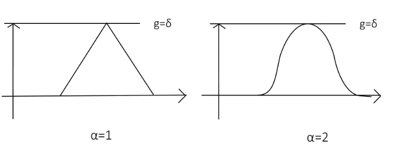
Figure 2: The left plot depicts a one dimensional density with gap of size at level λ. It is clear that {λ < p ≤ λ+} is an empty set. The right plot depicts 500 i.i.d sampling from a two dimensional density with a gap. It is clear that the density is low in the background and high in the disk centered at (-1,-1) and in the square centered at (1,1). Finding the samples points with low density values can be thought of as outliers detection in this case.
Though fairly restrictive, the scenario of a distribution with a gap is quite interesting for the purpose of both clustering and level set estimation. Indeed, this situation encom-passes the ideal clustering scenario, depicted as examples in Figures 1 and 5 in the original DBSCAN paper Ester et al. (1996), of a piece-wise constant density that is low everywhere on its support with the exception of a few connected, full-dimensional regions, or clusters, where it is higher by a certain amount (in our case the gap). The size of the gap parameter and the minimal distance among clusters both affect the difficulty of the clustering task, which becomes harder as the parameters get smaller.
To formally capture the dependence on the distance between clusters we set
Sλ∗ = I
[
i=1 Ci,
where (C1, . . . ,CI) are disjoint, connected, (necessarily) closed sets of positive P measure and let
σ = min
i6=j dist(Ci,Cj)>0 (23)
the separation parameter σ vary with n (though we do not make this dependence in out notation for ease of readability), thus allowing for harder clustering problems as a function of the sample size.
In the next simple result, we show that a flat version of the vanilla DBSCAN algorithm given in Algorithm 1, with suitable choices for the input parameters, can optimally estimate the clusters at λ∗ at a rate that depend explicitly on both andσ.
Proposition 4. Let {X1, . . . , Xn}be an i.i.d. sample from a probability distribution P that
has a gap of size at levelλ∗. Setan=C1
q
log(n)+log(1/h)
nhd as in (7) and suppose the input
parameters h and k of the DBSCAN algorithm are such that
σ/4≥h≥C
log(n) n2
1/d
and k=dnhdVdλe, (24)
for anyC >0 such that2an< and any λin (λ∗−+an, λ∗−an]. Then with probability
at least 1−1/n:
i. simultaneously over all connected setsAsuch thatA2h⊂ Ci, for somei, all the sample
points in A, if any, belong to the same connected component of Gk,h;
ii. simultaneously over all connected sets A and A0 such that A2h ⊂ Ci and A02h ⊂ Cj,
for some i 6= j, the sample points in A and A0, if any, belong to distinct connected components ofGk,h.
The definition of A2h andA−2h can be found in (1). Notice that the above results hold
true for allnlarge enough such thatan< /2. Proposition 4 implies the DBSCAN algorithm
will yield clustering consistency, in the sense of Chaudhuri et al. (2014), provided that its input parameters fulfill (24) holds. In particular, this result requires that the sample size relates to the gap parameterand the separation parameter σ according to the inequality
n≥C 1 2σd,
for some constant C, depending ond. In fact, such scaling is nearly minimax optimal: no other clustering algorithms can guarantee cluster consistency under the same assumptions and with a better sample complexity as a function of both and σ. This results follows from the lower bound guarantee given in Theorem VI.1 of Chaudhuri et al. (2014), where we take notice that the parameters σ and have different, though related, meaning; see Appendix C.4. In fact, the results in Proposition 4 can be further extended to hold over more general settings of arbitrary densities; see Appendix D.
5.1. The Devroye-Wise estimator of the Level Sets
The assumption of a density with gap allows us to carry out a further analysis of the DBSCAN algorithm, showing that it is also minimax optimal for estimating the level set itself Sλ∗. For this purpose, the DBSCAN algorithm reduces to the renown Devroye-Wise
estimator: see Devroye and Wise (1980). Below we provide a novel, sharper analysis of this estimator, where we allow the size of the gap to decrease with n, and demonstrate that its rate-optimal (again, we will not explicitly express this dependence in our notation for simplicity). To the best of our knowledge, such scaling has not been previously established. Recall that the DBSCAN algorithm with inputs k and h outputs a set of nodes Gh,k.
One then may construct the estimator
b Sh =
[
Xj∈Gh,k
B(Xj, h) (25)
comprised of a union of balls around such points, and use it as an estimator of the corre-sponding high density region S=Sλ∗ =∪I
i=1Ci consisting of all the clusters.
We measure the performance of any estimator Sb with the Lebesgue measure of its symmetric difference withS:
LS∆Sb
=LS∩Sbc
+LSc∩Sb
.
We will in addition impose the following condition:
R. (Level set regularity). There exists constants h0 >0 and C0 > 0 such that, for all
h∈(0, h0),
L(Sh\S−h)≤C0h,
whereSh and S−h are defined in (1).
ConditionRis very mild. Indeed, if∂SisC2, then the setNh:=Sh\S−h is the tubular
neighborhood (see, e.g. Hirsch, 2012) of ∂S inRd. In particular, every compact domain in RdwithC2 boundary satisfies conditionR. In this case C0 Vd−1|∂S|, where|∂S|denotes
the surface volume of S. We also note that R is equivalent to the “smooth boundary” condition in Steinwart (2015).
Proposition 5. Let {X1, . . . , Xn}be an i.i.d. sample from a probability distribution P that
has a gap of size at level λ∗. Let an=C
q
log(n)+log(1/h)
nhd be defined as in (7). Suppose the
input parameters (h, k) of the DBSCAN algorithm satisfy
h0 ≥h≥C
log(n)
n2
1/d
and k=dnhd, Vdλe (26)
for anyC >0 such that2an< and any λin (λ∗−+an, λ∗−an]. Then with probability
at least 1−1/n,
L(S4Sbh)≤2C0h,
where C0 is defined in R and
b Sh =
[
Xj∈Gh,k
Similarly to Proposition 4, the above results hold true for all nlarge enough such that an < /2. If P(X ∈ S) = 1, the level set estimator Sbh is also a support estimator and = infx∈Sp(x). In this case, Proposition 5 says that if the lower bound on the density
vanishes no faster thanO(n−1/2), then support estimation is still possible.
Below we show that the error bound given in Proposition 5 is minimax optimal up to log factors. Consider Pn(h
0, ), the class of probability distribution of n i.i.d. random vectors
in Rd whose common density exhibit a gap of size such that condition (22) holds, and
satisfying condition R with parameter h0 > 0. Then Proposition 5 shows that, for all n
large enough,
sup
P∈Pn(h0,)EP
S4Sbh
=O
log(n)
n2
1/d! ,
provided that h is of the order
log(n)
n2
1/d
. Our next result provides a nearly-matching lower bound.
Proposition 6. There exist constants h0 and c, depending only on d such that for any
≤1/4, for allnlarge enough here exist probability distributions {P1, . . . , PM}in Pn(h0, ) such that
inf b
S
sup
i=1,...,M
EPi
L(Sb4S)
≥cmin (
1 n2
1/d ,1
)
,
where the infimum is with respect to all estimators of S.
Thus, if log(n2n) →0 as n → ∞ (so that condition (26) is eventually satisfied), then the
bounds given in Proposition 5 and Proposition 6 match, up to a log(n) factor. That is, with suitable choice of input, DBSCAN can optimally estimate the level setS at the gap.
The performance of the Devroye-Wise estimator is a well-established topic in the liter-ature: see, e.g., Theorem 4 and 5 in Cuevas and Rodr´ıguez-Casal (2004). Our contribution in this regard is two fold: we allow for an explicit dependence on the gap size parameter and deliver minimax lower bounds. Our rate of convergence confirms the intuition that a smaller gap size leads to a harder estimation problem.
6. Discussion
6.1. Hartigan consistency in Hartigan (1981)
We follow Chaudhuri and Dasgupta (2010) and Eldridge et al. (2015) in defining Hartigan consistency in terms of the density cluster tree.
Definition 8 (Hartigan consistency). Let Tbn be a cluster tree estimator constructed from
i.i.d. data {Xi}ni=1 from a disribution P with Lebesgue density p. For any pair of subsets
A and A0, let denote An and A0n be the smallest clusters of Tbn containing A∩ {Xi}ni=1 and A0∩ {Xi}ni=1, respectively. The cluster tree estimator Tbn is Hartigan consistent if, for any
pair of setsA andA0 belonging to distinct connected components of{x:p(x)≥λ} for some
λ,P(An∩An0 =∅)→1 as n→ ∞.
It is immediate from Definition 3 that a δ-consistent cluster tree is also Hartigan con-sistent. While Hartigan consistency is a simple form of point-wisecluster tree consistency, which holds for each fixed pairs of disjoint clusters, δ-consistency is a stronger guaran-tee, as it yields uniform consistency over all δ-separated clusters and, furthermore, gives consistency rates depending on the value of the separation parameterδ.
6.2. Comparison with the Merge distortion metric
The notion ofδ-separation is closely related to the notion of merge distance introduced by Eldridge et al. (2015), which we present next.
Definition 9. Letpandqbe Lebesgue densities inRdand letTp andTqbe the corresponding
cluster density trees. The merge distortion distance between Tp and Tq is defined as
dM(Tp, Tq) = sup x,y∈Rd
|mp(x, y)−mq(x, y)|,
where, for a Lebesgue density p,
mp(x, y) = sup{λ >0∈R:there exists C∈Tp(λ) such that {x, y} ⊂C}.
The original definition of merge distortion metric is, in fact, more general but, when specialized to our settings, reduces to the one given above.
The merge distortion distance is closely related to the L∞ distance between densities. In fact, by Theorem 17 in Eldridge et al. (2015), dM(Tp, Tq)≤ kp−qk∞, so that, if {pn}n
is a sequence of Lebesgue densities, then kpn−pk → 0 implies that dM(Tpn, Tp) → 0. In
fact, Lemma 1 in Appendix F of Kim et al. (2016) shows that, if p and q are continuous, then dM(Tp, Tq) = kp−qk∞. As a result, for the class of continuous (and, in particular,
H¨older smooth) densities, cluster consistency in the merge distortion distance is equivalent to cluster consistency based on the δ-separation criterion, which in turn is equivalent to estimation consistency of the underlying density in theL∞ norm.
The above statement immediately applies to the n¨aive cluster tree estimatorT b
phn built
using the level sets of any density estimator pbhn that is continuous and, as hn → ∞,
is sufficient to demonstrate the properties of minimality and separation, as defined in that reference, for the DBSCAN cluster-tree estimators. The separation property, which prevents the emergence of false clusters or over-segmentation, follows directly from the definition ofδ -separation; see also the pruning results of Section 4.6. On the other hand, minimality avoids the occurrence of improper nesting and holds for the DBSCAN procedures we consider here in virtue of Lemma 1 and Lemma 6. The fact that our algorithms produce cluster tree estimators that are consistent in the merge distance should not be surprising, since δ -consistency is directly tied to -consistency for density estimation in in L∞. As shown in Eldridge et al. (2015), the robust single-linkage clustering algorithm of Chaudhuri et al. (2014) is also consistent in the merge distance.
6.3. Comparison with the (, σ)-separation criterion of Chaudhuri et al. (2014)
The criterion ofδ-separation we introduce in this paper is most useful when studying smooth densities. Nonetheless, it will be helpful to compare it to the notion of (, σ)-separation defined in Chaudhuri et al. (2014), which is applicable to arbitrary densities.
Definition 10 ((, σ)-separation criterion in Chaudhuri et al. (2014)).
1. Let f be a density supported on X ⊂Rd. We say that A, A0 ⊂X are (, σ)-separated
if there exists S ⊂ X (the separator set) such that (i) any path in X from A to A0
intersects S, and (ii) supx∈Sσf(x)<(1−) infx∈Aσ∪A0σf(x).
2. Suppose an i.i.d samples {Xi}ni=1 is given. An estimate of the cluster tree is said to be(, σ)consistent if for any pair AandA0 being(, σ)separated, the smallest cluster containing A∩ {Xi}ni=1 is disjoint from the smallest cluster containing A0∩ {Xi}ni=1.
In the following result we make a straightforward connection between the δ-separation and (, σ)-separation.
Lemma 3. Assume that p∈Σ(L, α) withα≤1 and that A andA0 are δ-separated. Then,
A and A0 are (, σ)-separated with
S ={x:p(x)≤λ−δ}, =δ/(3λ) and σα =δ/(3L), (28)
where λ= infz∈A∪A0p(z).
Proof of lemma 3. Denote λ = infz∈A∪A0p(z). Suppose for the sake of contradiction that
there is a path l connects A and A0 and that l∩ {p ≤ λ−δ} = ∅. Then by the conti-nuity of p and the compactness of l, there exist γ > 0 such that l ⊂ {p ≥ λ−δ+γ}. Thus A and A0 belongs to the same path connected component of {p ≥λ−δ+γ}. Since
{p≥λ−δ+γ} ⊂ {p > λ−δ},A and A0 belongs to the same path connected component of {p > λ}. Since {p > λ} is an open set, A and A0 be belongs to the same connected component of{p > λ}. This is a contradiction.
Let σα = δ/(3L) and = δ/3, then for any x ∈ Sσ, p(x) ≤ λ−δ +Lσα = λ−2δ/3.
Similarly if x∈Aσ∪A0σ,p(x)≥λ−Lσα =λ−δ/3. Thus
(1−) inf
x∈Aσ∪A0σ
f(x)>(1−)λ−δ/3 =λ−2δ/3> sup
x∈Sσ
According to the separation criterion in Definition 10, two clusters can be (, σ)-separated for many the values ofand σ. In particular, by taking the separator set to be larger, it is easy to produce examples ofδ-separated clusters that are also (, σ)-separated such thatδ is big butσis small. This is simply becauseσ is heavily associated withS. And conversely, by taking an almost flat density function, it is possible to have a very largeσ and very small δ.
We remark that when α > 1, there is no obvious relationship between the parameter (σ, ) in Definition 10 andδin Definition 3 as that in Lemma 3. Forα >1, whilep∈Σ(L, α) implies thatp is Lipschitz continuous, the Lipschitz constant in this case does not depend on L and α in a simple manner. As a result, the parameter σ, representing the distance between connected components of upper level sets ofp, is not straightforwardly related to δ.
References
Ery Arias-Castro, David Mason, and Bruno Pelletier. On the estimation of the gradient lines of a density and the consistency of the mean-shift algorithm. Journal of Machine Learning Research, 17(1):1487–1514, 2016.
Amparo Ba´Illo, Antonio Cuevas, and Ana Justel. Set estimation and nonparametric detec-tion. Canadian Journal of Statistics, 28(4):765–782, 2000.
Sivaraman Balakrishnan, Srivatsan Narayanan, Alessandro Rinaldo, Aarti Singh, and Larry Wasserman. Cluster trees on manifolds. In Advances in Neural Information Processing Systems, 2012.
Jos´e E Chac´on. A population background for nonparametric density-based clustering. Sta-tistical Science, 30(4):518–532, 2015.
Kamalika Chaudhuri and Sanjoy Dasgupta. Rates of convergence for the cluster tree. In
Advances in Neural Information Processing Systems, pages 343–351, 2010.
Kamalika Chaudhuri, Sanjoy Dasgupta, Samory Kpotufe, and Ulrike von Luxburg. Con-sistent procedures for cluster tree estimation and pruning. IEEE Transactions on Infor-mation Theory, 60(12):7900–7912, 2014.
Fr´ed´eric Chazal, Marc Glisse, Catherine Labru`ere, and Bertrand Michel. Convergence rates for persistence diagram estimation in topological data analysis. Journal of Machine Learning Research, 16(1):3603–3635, 2015.
Yen-Chi Chen, Christopher R Genovese, and Larry Wasserman. Density level sets: Asymp-totics, inference, and visualization. Journal of the American Statistical Association, 112 (520):1684–1696, 2017.
Antonio Cuevas. Set estimation: Another bridge between statistics and geometry. Bolet´ın de Estad´ıstica e Investigaci´on Operativa, 25(2):71–85, 2009.
Antonio Cuevas and Alberto Rodr´ıguez-Casal. On boundary estimation. Advances in Ap-plied Probability, 36(2):340–354, 2004.
Luc Devroye and Gary L. Wise. Detection of abnormal behavior via nonparametric esti-mation of the support. SIAM Journal on Applied Mathematics, 38(3):480–488, 1980.
Manfredo Perdigao Do Carmo. Riemannian geometry. Birkhauser, 1992.
Justin Eldridge, Mikhail Belkin, and Yusu Wang. Beyond hartigan consistency: Merge distortion metric for hierarchical clustering. In Proceedings of The 28th Conference on Learning Theory, pages 588–606, 2015.
Martin Ester, Hans-Peter Kriegel, J¨org Sander, Xiaowei Xu, et al. A density-based algo-rithm for discovering clusters in large spatial databases with noise. InProceedings of the Second International Conference on Knowledge Discovery and Data Mining, Kdd, pages 226–231, 1996.
Junhao Gan and Yufei Tao. Dbscan revisited: Mis-claim, un-fixability, and approximation. In Proceedings of the 2015 ACM SIGMOD International Conference on Management of Data, SIGMOD ’15, 2015.
Evarist Gin´e and Armelle Guillou. Rates of strong uniform consistency for multivariate kernel density estimators. Annales de l’IHP Probabilit´es et statistiques, 38:907–921, 2002.
John A Hartigan. Consistency of single linkage for high-density clusters. Journal of the American Statistical Association, 76(374):388–394, 1981.
Morris W Hirsch. Differential topology, volume 33. Springer Science & Business Media, 2012.
Jennifer Jang and Heinrich Jiang. Dbscan++: Towards fast and scalable density clustering.
arXiv preprint arXiv:1810.13105, 2018.
Heinrich Jiang. Density level set estimation on manifolds with dbscan. arXiv preprint arXiv:1703.03503, 2017a.
Heinrich Jiang. Uniform convergence rates for kernel density estimation. In International Conference on Machine Learning, pages 1694–1703, 2017b.
Heinrich Jiang, Jennifer Jang, and Ofir Nachum. Robustness guarantees for density cluster-ing. InThe 22nd International Conference on Artificial Intelligence and Statistics, pages 3342–3351, 2019.
Jisu Kim, Yen-Chi Chen, Sivaraman Balakrishnan, Alessandro Rinaldo, and Larry Wasser-man. Statistical inference for cluster trees. InAdvances in Neural Information Processing Systems 29, pages 1839–1847. 2016.
Jussi Klemel¨a. Complexity penalized support estimation. Journal of multivariate analysis, 88(2):274–297, 2004.
Jussi Klemel¨a. Smoothing of Multivariate Data: Density Estimation and Visualization. Wiley, 2009.
Aleksandr Petrovich Korostelev and Alexandre B Tsybakov. Minimax theory of image reconstruction, volume 82. Springer Science & Business Media, 1993.
Samory Kpotufe and Ulrike V Luxburg. Pruning nearest neighbor cluster trees. In Pro-ceedings of the 28th International Conference on Machine Learning (ICML-11), pages 225–232, 2011.
James R Munkres. Topology. Prentice Hall, 2000.
Deborah Nolan and David Pollard. U-processes: rates of convergence. The Annals of Statistics, pages 780–799, 1987.
Mathew D. Penrose. Single linkage clustering and continuum percolation. Journal of Mul-tivariate Analysis, 53:94–109, 1995.
Wolfgang Polonik. Measuring mass concentrations and estimating density contour clusters-an excess mass approach. The Annals of Statistics, pages 855–881, 1995.
Philippe Rigollet and R´egis Vert. Optimal rates for plug-in estimators of density level sets.
Bernoulli, pages 1154–1178, 2009.
Alessandro Rinaldo and Larry Wasserman. Generalized density clustering. The Annals of Statistics, pages 2678–2722, 2010.
Alessandro Rinaldo, Aarti Singh, Rebecca Nugent, and Larry Wasserman. Stability of density-based clustering. The Journal of Machine Learning Research, 13:905–948, 2012.
Arrti Singh, Clayton Scott, Robert Nowak, and Aarti Singh. Adaptive hausdorff estimation of density level sets. The Annals of Statistics, 37:2760–2782, 2009.
Bharath K Sriperumbudur and Ingo Steinwart. Consistency and rates for clustering with dbscan. In AISTATS, pages 1090–1098, 2012.
Ingo Steinwart. Adaptive density level set clustering. In Proceedings of the 24th Annual Conference on Learning Theory, pages 703–738, 2011.
Ingo Steinwart. Fully adaptive density-based clustering. The Annals of Statistics, 43(5): 2132–2167, 2015.
Ingo Steinwart, Bharath K. Sriperumbudur, and Philipp Thomann. Adaptive clustering using kernel density estimators. arXiv preprint arXiv:1708.05254, 2017.
Werner Stuetzle and Rebecca Nugent. A generalized single linkage method for estimating the cluster tree of a density. Journal of Computational and Graphical Statistics, 19(2), 2010.
Alexandre B Tsybakov.Introduction to nonparametric estimation. Springer Series in Statis-tics, 2009.
Alexandre B Tsybakov et al. On nonparametric estimation of density level sets.The Annals of Statistics, 25(3):948–969, 1997.
Bingchen Wang, Chenglong Zhang, Lei Song, Lianhe Zhao, Yu Dou, and Zihao Yu. Design and optimization of dbscan algorithm based on cuda. arXiv preprint arXiv:1506.02226, 2015.
RM Willett and Robert D Nowak. Minimax optimal level-set estimation.IEEE Transactions on Image Processing, 16(12):2965–2979, 2007.
Appendix A. Topological Preliminaries
For completeness, we review the definition of connectedness from the general topology.
Definition 11 ( Munkres (2000) Chapter 3). LetU be any nonempty subset inRd. ThenU is said to be connected, if, for every pair of open subsetsA, A0 ofU such thatA∪A0=U, we have either A=∅ or A0 =∅. The maximal connected subsets of U are called the connected components ofU.
We briefly explain why the connected components naturally introduce a hierarchical structure to the level sets ofp. Letλ1 > λ2, so we have {p≥λ1} ⊂ {p≥λ2}.
• Suppose A is any subset of Rd, and A belongs to the same connected component of {p≥λ1}. Then Ais contained in the same connected component of {p≥λ2}. • Suppose A∪A0 ⊂ {p ≥ λ1} and they belong to distinct connected components of
{p ≥ λ2} Then A and A0 are not contained in the same connected component of {p≥λ1}.
We also review a closed related concepts, which is call the path connectedness in general topology.
Definition 12. We say that a subset U ⊂Rd is path connected if for any x, y∈ U, there
exists a path continuous P : [0,1]→U such that P(0) =x andP(1) =y.
The main reason we introduce the path connectedness is that if U is an open set in
Rd, then U is connected if and only if it is path connected. Therefore a simple but useful
consequence is that for any λ, the connected components of {p > λ} are also the path connected components.