Shared Subspace Models for Multi-Group Covariance
Estimation
Alexander M. Franks [email protected]
Department of Probability and Applied Statistics Statistics University of California, Santa Barbara
Santa Barbara, CA 93106, USA
Peter Hoff [email protected]
Department of Statistical Science Duke University
Durham, NC 27708, USA
Editor:Barbara Engelhardt
Abstract
We develop a model-based method for evaluating heterogeneity among several p×p
covariance matrices in the large p, small n setting. This is done by assuming a spiked covariance model for each group and sharing information about the space spanned by the group-level eigenvectors. We use an empirical Bayes method to identify a low-dimensional subspace which explains variation across all groups and use an MCMC algorithm to es-timate the posterior uncertainty of eigenvectors and eigenvalues on this subspace. The implementation and utility of our model is illustrated with analyses of high-dimensional multivariate gene expression.
Keywords: covariance estimation; spiked covariance model; Stiefel manifold; large p, smalln; high-dimensional data; empirical Bayes; gene expression data.
1. Introduction
Multivariate data can often be partitioned into groups, each of which represent samples from populations with distinct but possibly related distributions. Although historically the primary focus has been on identifying mean-level differences between populations, there has been a growing need to identify differences in population covariances as well. For instance, in case-control studies, mean-level effects may be small relative to subject variability; dis-tributional differences between groups may still be evident as differences in the covariances between features. Even when mean-level differences are detectable, better estimates of the covariability of features across groups may lead to an improved understanding of the mechanisms underlying these apparent mean-level differences. Further, accurate covariance estimation is an essential part of many prediction tasks (e.g. quadratic discriminant anal-ysis). Thus, evaluating heterogeneity between covariance matrices can be an important complement to more traditional analyses for estimating differences in means across groups. To address this need, we develop a novel method for multi-group covariance estimation. Our method exploits the fact that in many natural systems, high dimensional data is often
very structured and thus can be best understood on a lower dimensional subspace. For example, with gene expression data, we may be interested how the covariability between expression levels differs in subjects with and without a particular disease phenotype (e.g, how does gene expression covariability differ in different subtypes of leukemia? See Section 6). In these applications, the effective dimensionality is thought to scale with the number of gene regulatory modules, not the number of genes themselves (Heimberg et al., 2016). As such, differences in gene expression across groups should be expressed in terms of differences between these regulatory modules rather than strict differences between expression levels. Such differences can be examined on a subspace that reflects the correlations resulting from these modules. In contrast to most existing approaches for group covariance estimation, our approach is to directly infer such subspaces from groups of related data.
Some of the earliest approaches for multi-group covariance estimation focus on estima-tion in terms of spectral decomposiestima-tions. Flury (1987) developed estimaestima-tion and testing procedures for the “common principal components” model, in which a set of covariance matrices were assumed to share the same eigenvectors. Schott (1991, 1999) considered cases in which only certain eigenvectors are shared across populations, and Boik (2002) described an even more general model in which eigenvectors can be shared between some or all of the groups. More recently, Hoff (2009a), noting that eigenvectors are unlikely to be shared exactly between groups, introduced a hierarchical model for eigenvector shrinkage based on the matrix Bingham distribution. There has also been a significant interest in estimating covariance matrices using Gaussian graphical models. For Gaussian graphical models, zeros in the precision matrix correspond to conditional independence relationships between pairs of features given the remaining features (Meinshausen and B¨uhlmann, 2006). Danaher et al. (2014) extended existing work in this area to the multi-group setting, by pooling information about the pattern of zeros across precision matrices.
Another popular method for modeling relationships between high-dimensional multi-variate data is partial least squares regression (PLS) (Wold et al., 2001). This approach, which is a special case of a bilinear factor model, involves projecting the data onto a lower dimensional space which maximizes the similarity of the two groups. This technique does not require the data from each group to share the same feature set. A common variant for prediction, partial least squares discriminant analysis (PLS-DA) is especially common in chemometrics and bioinformatics (Barker and Rayens, 2003). Although closely related to the approaches we will consider here, the primarily goal of PLS-based models is to create regression or discrimination models, not to explicitly infer covariance matrices from multi-ple groups of data. Nevertheless, the basic idea that data can often be well represented on a low dimensional subspace is an appealing one that we leverage.
In this paper we propose a multi-group covariance estimation model by sharing infor-mation about the subspace spanned by group-level eigenvectors. Our approach is closely related to the covariance reducing model proposed by Cook and Forzani (2008), but their model is applicable only whennp. In this work we focus explicitly on high-dimensional inference in the context of the “the spiked covariance model” (also known as the “partial isotropy model”), a well studied variant of the factor model (Mardia et al., 1980; Johnstone, 2001). Unlike most previous methods for multi-group covariance estimation, our shared subspace model can be used to improve high-dimensional covariance estimates, facilitates exploration and interpretation of differences between covariance matrices, and incorporates uncertainty quantification. It is also straightforward to integrate assumptions used in pre-vious approaches (e.g. eigenvector shrinkage) to the shared subspace model.
In Section 2 we briefly review the behavior of spiked covariance models for estimating a single covariance matrix and then introduce our extension to the multi-group setting. In Section 3 we describe an efficient empirical Bayes algorithm for inferring the shared subspace and estimating the posterior distribution of the covariance matrices of the data projected onto this subspace. In Section 4 we investigate the behavior of this class of models in simulation and demonstrate how the shared subspace assumption is widely applicable, even when there is little similarity in the covariance matrices across groups. In particular, independent covariance estimation is equivalent to shared subspace estimation with a suffi-ciently large shared subspace. In Section 5 we use an asymptotic approximation to describe how shared subspace inference reduces bias when bothpandnare large. Finally, In Section 6 we demonstrate the utility of a shared subspace model in an analysis of gene expression data from juvenile leukemia patients . Despite the large feature size (p >3000) relative to the sample size (n < 100 per group), we identify interpretable similarities and differences in gene covariances on a low dimensional subspace.
2. A Shared Subspace Spiked Covariance Model
Suppose a random matrix S has a possibly degenerate Wishart(Σ, n) distribution with density given by
p(S|Σ, n)∝l(Σ :S) =|Σ|−n/2etr(−Σ−1S/2), (1) where etr is the exponentiated trace, the covariance matrix is a positive definite matrix, i.e. Σ ∈ S+
p , and n may be less than p. Such a likelihood results from S being, for example,
a residual sum of squares matrix from a multivariate regression analysis. In this case, nis the number of independent observations minus the rank of the design matrix.
In this paper we consider multi-group covariance estimation based on K matrices,
Y1, ..., YK, whereYkis assumed to be annkbypmatrix of mean-zero normal data, typically
withnk p. Then, YkTYk =Sk has a (degenerate) Wishart distribution as in Equation 1.
To improve estimation, we seek estimators of each covariance matrix, ˆΣk, that may depend
on data from all groups. Specifically, we posit that the covariance matrix for each group can be written as
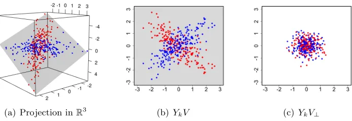
(a) Projection inR3 (b) YkV (c)YkV⊥
Figure 1: Two groups of four-dimensional data (red and blue) projected into different sub-spaces. a) To visualize Yk we can project the data into R3. In this
illustra-tion, the distributional differences between the groups are confined to a two-dimensional shared subspace (V VT, grey plane). b) The data projected onto the two-dimensional shared subspace, YkV, have covariances Ψk that differ between
groups. c) The orthogonal projection,YkV⊥ has isotropic covariance,σ2kI, for all
groups.
whereV is ap×ssemi-orthogonal matrix whose columns form the basis vectors for subspace of variation shared by all groups. Ψk is a non-isotropic s×s covariance matrix for each
group on this subspace of variation and it is assumed thatsp.
Our model extends the spiked principal components model (spiked PCA), studied ex-tensively by Johnstone (2001) and others, to the multi-group setting. Spiked PCA assumes that
Σ =σ2(UΛUT +I) (3) where for s p, Λ is an s×s diagonal matrix and U ∈ Vp,s, where Vp,s is the Stiefel
manifold consisting of all p×s semi-orthogonal matrices in Rp, so that UTU = Is. The
spiked covariance formulation is appealing because it explicitly partitions the covariance matrix into a tractable low rank “signal” and isotropic “noise”.
Classical results for parametric models (e.g., Kiefer and Schwartz (1965)) imply that asymptotically in n for fixed p, an estimator will be consistent for a spiked population covariance as long as the assumed number of spikes (eigenvalues larger thanσ2) is greater than or equal to the true number. However, when p is large relative to n, as is the case for the examples considered here, things are more difficult. Under the spiked covariance model, it has been shown that if p/n → α > 0 as n → ∞, the kth largest eigenvalue of
S/(nσ2) will converge to an upwardly biased version ofλk+ 1 ifλkis greater than √
Single-group covariance estimators of the spiked PCA form are equivariant with respect to rotations and scale changes, but the situation should be different, when we are interested in estimating multiple covariance matrices from distinct but related groups with shared features. Here, equivariance to distinct rotations in each group is an unreasonable assump-tion; both eigenvalue and eigenvector shrinkage can play an important role in improving covariance estimates.
In the multi-group setting, we account for similarity between group-level eigenvectors by positing that the anisotropic variability from each group occurs on a common low di-mensional subspace. Throughout this paper we will denote to the shared subspace as
V VT ∈ Gp,s, whereGp,s is the Grassmannian manifold consisting of alls-dimensional linear
subspaces ofRp (Chikuse, 2012). AlthoughV is only identifiable up to right rotations, the
matrix V VT, which defines the plane of variation shared by all groups, is identifiable for a fixed dimension, s. To achieve the most dimension reduction, we target the shared sub-space of minimal dimension, e.g. the shared subsub-space for which all Ψk are full rank. Such
a minimal subspace is known as the central subspace (Cook, 2009). Later, to emphasize the connection to the spiked PCA model (3), we will write Ψk in terms of its
eigendecom-position, Ψk = OkΛkOk, where Ok are eigenvectors and Λk are the eigenvalues of Ψk (see
Section 3.2).
For the shared subspace model, VTΣkV = σk2(Ψk+I) is an anisotropic s-dimensional
covariance matrix for the projected data, YkV. In contrast, the data projected onto the
orthogonal space,YkV⊥, is isotropic for all groups. In Figure 1 we provide a simple
illustra-tion using simulated 4-dimensional data from two groups. In this example, the differences in distribution between the groups of data can be expressed on a two dimensional sub-space spanned by the columns of V ∈ V4,2. Differences in the correlations between the two groups manifest themselves on this shared subspace, whereas only the magnitude of the isotropic variability can differ between groups on the orthogonal space. Thus, a shared sub-space model can be viewed as a covariance partition model, where one partition includes the anisotropic variability from all groups and the other partition is constrained to the isotropic variability from each group. This isotropic variability is often characterized as measurement noise.
3. Empirical Bayes Inference
In this section we outline an empirical Bayes approach for estimating a low-dimensional shared subspace and the covariance matrices of the data projected onto this space. As we discuss in Section 4, if the spiked covariance model holds for each group individually, then the shared subspace assumption also holds, where the shared subspace is simply the span of the group-specific eigenvectors, U1, ..., UK. In practice, we can usually identify a
algorithm (Lindstrom and Bates, 1988). In many settings such an approach yields group-level inferences that are close to that which would be obtained if the correct across-groups model were known (see for example Efron and Morris, 1973). In Section 3.1 we describe the expectation-maximization algorithm for estimating the maximum marginal likelihood of the shared subspace, V VT. This approach is computationally tractable for high-dimensional data sets. Given an inferred subspace, we then seek estimators for the covariance matrices of the data projected onto this space. Because seemingly large differences in the point esti-mates of covariance matrices across groups may not actually reflect statistically significant differences, in Section 3.2 we also describe a Gibbs sampler that can be used to generate estimates of the projected covariance matrices, Ψk, and their associated uncertainty. Later,
in Section 4 we discuss strategies for inferring an appropriate value for s and explore how shared subspace models can be used for exploratory data analysis by visualizing covariance heterogeneity on two or three dimensional subspaces.
3.1. Estimating the Shared Subspace
In this section we describe a maximum marginal likelihood procedure for estimating the shared subspace, V VT, based on the expectation-maximization (EM) algorithm. The full
likelihood for the shared subspace model can be written as
p(S1, ...Sk|Σk, nk)∝ K
Y
k=1
|Σk|−nk/2etr(−Σ−k1Sk/2)
∝ K
Y
k=1
|Σk|−nk/2etr(−(σk2(VΨkVT +I))−1Sk/2)
∝ K
Y
k=1
|Σk|−nk/2etr(−
V(Ψk+I)−1/σk2VT + (I−V VT)/σk2
Sk/2)
∝ K
Y
k=1
(σk2)−nk(p−s)/2|M
k|−nk/2etr(−
V Mk−1VT + 1
σk2(I−V V
T)
Sk/2),
(4)
where we define Mk=σk2(Ψk+I). The log-likelihood in V (up to an additive constant) is
l(V) =X
k
tr −(V Mk−1VT +V VT/σk2)Sk/2
= 1 2
X
k
tr
( 1
σk2I −M
−1
k )V TS
kV
. (5)
We maximize the marginal likelihood ofV with an EM algorithm, whereMk−1 and σ12
k
are considered the “missing” parameters. We assume independent Jeffreys prior distributions for both σk2 and Mk. The Jeffreys prior distributions for these quantities correspond to
p(σk2) ∝1/σ2k and p(Mk) ∝ |Mk|−(s+1)/2. From the likelihood it can easily be shown that
the conditional posterior for Mk is
p(Mk|V)∝ |Mk|−(nk+s+1)/2etr(−(Mk−1V TS
Algorithm 1:Shared Subspace EM Algorithm
Initialize V0∈ Vp,s;
while ||Vt−Vt−1||F > do
E-step:
fork←1 to K do
φt(k) ←E[Mk−1|V(t−1)] =nk(V(Tt−1)SkV(t−1))−1;
τt(k)←E[σ12
k
|V(t−1)] = nk(p
−s)
tr[(I−V(t−1)V(Tt−1))Sk]
;
end M-step:
Vt←arg max V∈Vp,s
P
ktr
−(V φ(tk)VT +τt(k)V VT)Sk/2
;
end
which is an inverse-Wishart(VTS
kV, nk) distribution. The conditional posterior
distribu-tion ofσ2k is simply
p σ2|V∝(σk2)−nk(p−s)/2−1etr −(I−V VT)S
k/[2σ2k]
which is an inverse-gamma(nk(p−s)/2, tr[(I −V VT)Sk]/2) distribution. We summarize
our approach in Algorithm 1 below.
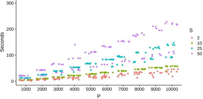
For the M-step, we use a numerical algorithm for optimization over the Stiefel manifold. The algorithm uses the Cayley transform to preserve the orthogonality constraints inV and has computationally complexity that is dominated by the dimension of the shared subspace, not the number of features (Wen and Yin, 2013). Specifically, the optimization routine has time complexity O(ps2 +s3), and consequently, our approach is computationally efficient for relatively small values ofs, even whenpis large. Run times are typically on the order of minutes for values of pas large as 10,000 and moderate values of s(e.g. <50). See Figure 10 in Appendix B for a plot with typical run times in simulations with a range of values of
p and s.
Initialization and Convergence: The Stiefel manifold is compact and the marginal
likelihood is continuous, so the likelihood is bounded. Thus, the EM algorithm, which increases the likelihood at each iteration, will converge to a stationary point (Wu, 1983). However, maximizing the marginal likelihood of the shared subspace model corresponds to a non-convex optimization problem over the Grassmannian manifold and may converge to a sub-optimal local mode or stationary point. Other work involving optimization on the Grassmannian has found convergence to non-optimal stationary values problematic and emphasized the importance of good (e.g. √n-consistent) starting values (Cook et al., 2016). Our empirical results on simulated data confirms that randomly initialized starting values converge to sub-optimal stationary values, and so in practice we initialize the algorithm at a carefully chosen starting value based on the eigenvectors of a pooled covariance estimate. We give the details for this initialization strategy below.
First, note that when the shared subspace model holds, the firstseigenvectors, fromany
ˆ
U(k)Uˆ(k)T is the eigenprojection matrix for the subspace spanned by the firstseigenvectors of Sk then it can be shown that
√
nvec( ˆU(k)Uˆ(k)T −V VT) converges in distribution to a mean-zero normal (Kollo, 2000). In the large p, small n setting, such classical asymptotic guarantees give little assurance that the resulting estimators would be reasonable, but they nevertheless suggest useful strategies for identifying starting value for the EM algorithm.
In this work, we choose a subspace initialization strategy based on sample eigenvectors of the data pooled from all groups. LetZ =P
kπkZσkk whereZkis a mean-zero normal with
covariance Σk andπk =nk/Pknk. ThenZ is a mixture of mean-zero normal distributions
with covariance
ΣZ =
X
k
πk
σ2kΣk
=VT(X
k
πk
σk2Ψk)V +I,
Clearly, the first s eigenvectors of ΣZ span the shared subspace, V VT. This suggests
that we can estimate the shared subspace using the scaled and pooled data, Ypool = [σ1
1Y1;
1 σ2Y2;...;
1
σkYk], where Ypool has dimension (
P
knk)×p. We use ˆUpoolUˆpoolT as the initial value for subspace estimation algorithm where ˆUpool are the first s eigenvectors of
Spool=YpoolT Ypool. If we treatYpoolas an i.i.d. sample from the mixture distributionZ, then it is known that ˆUpoolUˆpoolT is not consistent when both n and p growing at the same rate. For an arbitraryp-vectorη, the asymptotic bias ofηTUˆpoolUˆpoolT η is well characterized as a function of the eigenvalues of ΣZ(Mestre, 2008). If either the eigenvalues ofPkπσk2
k
Ψkor the
total sample size P
knk are large, ˆUpoolUˆpoolT will accurately estimate the shared subspace and likelihood based optimization may not be necessary. However, when either the eigen-values are small or the sample size is small the likelihood based analysis can significantly improve inference and ˆUpoolUˆpoolT is a useful starting value for the EM algorithm.
Evaluating Goodness of Fit: Tests for evaluating whether eigenvectors from multiple groups span a common subspace were explored extensively by Schott (1991). These tests can be useful for assessing whether a shared subspace model is appropriate, but cannot be used to test whether a particular subspace explains variation across groups. These results are also based on classical asymptotics and are thus less accurate when np
Our goodness of fit measure is based on the fact that when V is a basis for a shared subspace, then for each group, most of the non-isotropic variation inYkshould be preserved
when projecting the data onto this space. To characterize the extent to which this is true for different groups, we propose a simple estimator for the proportion of “signal” variance that lies on a given subspace. Specifically, we use the following statistic for the ratio of the sum of the firstseigenvalues of VTΣkV to the sum of the firstseigenvalues of Σk:
γ(Yk :V, σ2k) =
||YkV||2F/nk
max
e
V∈Vp,s
||YkVe||2F/nk−Bk
where||·||F is the Frobenius norm andBkis a bias correction whereBk=σk2p/nkPk
m(ik) m(ik)−σ2
k
withm(ik) the positive solution to the quadratic equation (m(ik))2+mi(k)(σk2p/nk−σk2−λˆ
(k) i )−λˆ
(k) i σ
2
k= 0. (7)
and ˆλ(ik) is the i-th eigenvalue ofSk/nk.
Theorem 1 Assumep/nk →αkandsis fixed. IfΣk=VΨkVT+σ2kI, thenγ(Yk:V, σk2) a.s → 1 as nk, p→ ∞.
Proof Since s is fixed and nk is growing, the numerator, ||YkV||2F/nk, is a consistent
estimator for the sum of the eigenvalues ofVTΣkV. In the denominator, max
e
V∈Vp,s
||YkVe||2F/nk
is equivalent to the sum of the first s eigenvalues of the sample covariance matrix Sk/nk.
Baik and Silverstein (2006) and others have demonstrated that asymptotically asp, nk→ ∞
and p/nk=αk, ˆλ(ik) is positively biased. Specifically,
ˆ
λ(ik) a.s.→ λ(ik) 1 + σ 2 kαk
λ(ik)−σ2k
!
(8)
Replacing λ(ik) by m(ik) and assuming equality in 8 yields the quadratic equation 7. The solution,m(ik), is an asymptotically (in nand p) unbiased estimator of λ(ik) and
max
e
V∈Vp,s
||YkVe||2F/nk−Bk
a.s. →
s
X
i
λ(ik) (9)
As such, when the shared subspace model holds both the numerator and denominator of the goodness of fit statistic converge almost surely to Ps
i=1λ (k)
i . Therefore γ(Yk :V, σk2) →1.
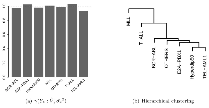
The goodness of fit statistic will be close to one for all groups when V VT is a shared subspace for the data and typically smaller if not. The metric provides a useful indicator of which groups can be reasonably compared on a given subspace and which groups cannot. In practice, we estimate a shared subspace ˆV and the isotropic variances ˆσk2 using EM and compute the plug-in estimate γ(Yk : ˆV ,σˆ2k). When this statistic is small for some groups,
it may suggest that the rank s of the inferred subspace needs to be larger to capture the variation in all groups. Ifγ(Yk: ˆV ,σˆ2k) is substantially larger than 1 for a particular group,
3.2. Inference for Projected Covariance Matrices
The EM algorithm presented in the previous section yields point estimates for V VT, Ψ k,
and σk2 but does not lead to natural uncertainty quantification for these estimates. In this section, we assume that the subspace V VT is fixed and known and demonstrate how we can estimate the posterior distribution for Ψk. Note that when the subspace is known, the
posterior distribution of Σk is conditionally independent from the other groups, so that we
can independently estimate the conditional posterior distributions for each group.
There are many different ways in which we could choose to parameterize Ψk. Building on
recent interest in the spiked covariance model (Donoho et al., 2013; Paul, 2007) we propose a tractable MCMC algorithm by specifying priors on the eigenvalues and eigenvectors of Ψk.
By modeling the eigenstructure, we can now view each covariance Σkin terms of the original
spiked principal components model. Equation 2, written as a function ofV, becomes
Ψk=OkΛkOkT
Σk=VΨkVT +σ2kI. (10)
Here, we allow Ψk to be of rank r≤sdimensional covariance matrix on thes-dimensional
subspace. Thus, Λk is anr×r diagonal matrix of eigenvalues, and Ok∈ Vs,r is the matrix
of eigenvectors of Ψk. For any individual group, this corresponds to the original spiked
PCA model (Equation 3) with Uk = V Ok ∈ Vp,r. Note that the V and Ok are jointly
unidentifiable because for any s×sorthonormal matrixW, V O=V WTW O= ˜VO˜. Once we fix a basis for the shared subspace, Ok is identifiable. As such, Ok should only be
interpreted relative to the basisV, as determined by the EM algorithm described in Section 3.1. Differentiating the ranks r and s is helpful because it enables us to independently specify a subspace common to all groups and the possibly lower rank features on this space that are specific to individual groups.
Although our model is most useful when the covariance matrices are related across groups, we can also use this formulation to specify models for multiple unrelated spiked covariance models. We explore this in detail in Section 4. In Section 6 we introduce a shared subspace model with additional structure on the eigenvectors and eigenvalues of Ψk
to facilitate interpretation of covariance heterogeneity on a two-dimensional subspace.
The likelihood for Σk given the sufficient statistic Sk = YkTYk is given in Equation 1.
For the spiked PCA formulation, we must rewrite this likelihood in terms ofV,Ok, Λk and
σk2. First note that by the Woodbury matrix identity
Σ−k1 = (σ2k(UkΛkUkT +I))−1
= 1
σ2 k
(UkΛkUkT +I)
−1
= 1
σk2(I−UkΩkU
T
where the diagonal matrix Ω = Λ(I+ Λ)−1, e.g. ωi= λiλ+1i . Further, |Σk|= (σk2)p|UkΛkUkT +I|
= (σk2)p|Λk+I|
= (σk2)p
r
Y
i=1
(λi+ 1)
= (σk2)p
r
Y
i=1
(1−ωi), (12)
where the second line is due to Sylvester’s determinant theorem. Now, the likelihood ofV,
Ok, Λk and σk2 is available from Equation 1 by substituting the appropriate quantities for
Σ−k1 and |Σk|and replacing Uk with V Ok:
L(σ2k, V, OkΩk:Yk)∝(σ2k)
−nkp/2etr(− 1
2σ2 k
Sk) r
Y
i=1
(1−ωki)
!nk/2
etr( 1 2σ2
k
(V OkΩkOTkVT)Sk).
(13) We use conjugate and semi-conjugate prior distributions for the parameters Ok, σ2k and
Ωk to facilitate inference via a Gibbs sampling algorithm. In the absence of specific prior
information, invariance considerations suggest the use of priors that lead to equivariant estimators. Below we describe our choices for the prior distributions of each parameter and the resultant conditional posterior distributions. We summarise the Gibbs Sampler in Algorithm 2.
Conditional distribution of σ2k: From Equation 13 it is clear that the inverse-gamma class of prior distributions is conjugate for σ2k. We chose a default prior distribution for σk2 that is equivariant with respect to scale changes. Specifically, we use the Jef-freys prior distribution, an improper prior with density p(σk2) ∝ 1/σk2. Under this prior, straightforward calculations show that the full conditional distribution of σ2k is inverse-gamma(nkp/2,tr[Sk(I−UkΩkUkT)/2]), where Uk=V Ok.
Conditional distribution of Ok: Given the likelihood from Equation 13, it is easy to
show that the class of Bingham distributions are conjugate forOk (Hoff, 2009a,b). Again,
invariance considerations lead us to use a rotationally invariant uniform probability measure on Vs,p. Under this uniform prior, the full conditional distribution of Ok has a density
proportional to the likelihood
p(Ok|σk2, Uk,Ωk)∝etr(ΩkOTkVT[Sk/(2σk2)]V Ok). (14)
This is a Bingham(Ω, VTSkV /(2σ2)) distribution on Vs,r (Khatri and Mardia, 1977). A
Gibbs sampler to simulate from this distribution is given in Hoff (2009b).
Together, the prior forσk2andOkleads to conditional (onV) Bayes estimators ˆΣ(VTSkV)
that are equivariant with respect to scale changes and rotations on the subspace spanned by
V, so that ˆΣ(aW VTSkV WT) =aWΣ(ˆ VTSkV)W for all a >0 and W ∈ Os (assuming an
invariant loss function). Interestingly, if Ωk were known (which it is not), then for a given
Algorithm 2:Gibbs Sampler for Projected Data Covariance Matrices
Estimate ˆV using EM (Algorithm 1). Initialize Ok,Λk, σk2;
for s←1 to number of samplesdo
fork←1 to K do
Sampleσk2 from an inverse-gamma(nkp/2,tr[Sk(I−V Oˆ kΩkVˆTOTk)/2]);
SampleOk from a Bingham(Ω,VˆTSkV /ˆ (2σ2));
fori←1 to r do
Sample (1−ωki) from a gamma(nk/2 + 1, ckink/2) truncated at 1;
λki ←ωki/(1−ωki)
end end end
Conditional distribution for Ωk: Here we specify the conditional distribution of the
diagonal matrix Ωk = Λk(I+ Λk)−1 = diag(ωk1, ...ωkr). We consider a uniform(0,1) prior
distribution for each element of Ω, or equivalently, anF2,2prior distribution for the elements of Λ. The full conditional distribution of an elementωi of Ω is proportional to the likelihood
function
p(ωki|V, Ok, Sk)∝ωki
r
Y
i=1
(1−ωki)nk/2
!
etr( 1 2σ2
k
(V OkΩkOTkVT)Sk) (15)
∝(1−ωki)nk/2eckiωkink/2, (16)
wherecki =uTkiSkuki/(nkσk2) anduki is columniofUk=V Ok. It is straightforward to show
that the density for (1−ωki) is proportional to a gamma(nk/2 + 1, ckink/2) truncated at 1.
Thus, we can easily sample from this distribution using inversion sampling. The behavior of the distribution for ωki is straightforward to understand: if cki ≤ 1, then the function
has a maximum at ωki = 0, and decays monotonically to zero as ωki →1. If cki >1 then
the function is uniquely maximized at (cki−1)/cki ∈(0,1). To see why this makes sense,
note that the likelihood is maximized when the columns ofUkare equal to the eigenvectors
of Sk corresponding to its top r eigenvalues (Tipping and Bishop, 1999). At this value of
Uk,cki will then equal one of the topr eigenvalues ofSk/(nkσk2). In the case thatnkp,
we expect Sk/(nkσk2) ≈ Σk/σ2k, the true (scaled) population covariance, and so we expect
cki to be near one of the top r eigenvalues of Σk/σk2, sayλki+ 1. If indeed Σk hasr spikes,
then λki > 0, cki ≈ λki + 1 > 1, and so the conditional mode of wki is approximately
(cki−1)/cki=λki/(λki+ 1), the correct value. On the other hand, if we have assumed the
existence of a spike when there is none, then λki = 0, cki ≈ 1 and the Bayes estimate of
wki will be shrunk towards zero, as it should be. We summarise the full Gibbs sampling
algorithm below.
4. Simulation Studies
subspace. Here, we simulateK = 5 groups of data from the shared subspace spiked covari-ance model with p = 20000 features, a shared subspace dimension of s = r = 2, σ2k = 1, and nk = 100. We fix the first eigenvalue of Ψk from each group to λ1 = 1000 and vary
λ2. We generate the basis for the shared subspace and the eigenvectors of Ψk by sampling
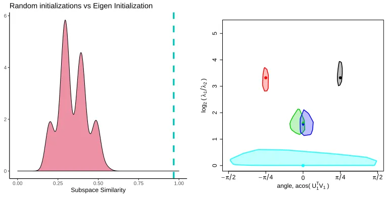
uniformly from the Stiefel manifold. First, in Figure 2(a) we demonstrate the importance of the eigen-based initialization strategy proposed in Section 3.1. As an accuracy metric, we study the behavior of tr( ˆVVˆTV VT)/s which is bounded by zero and one and achieves a maximum of one if and only if ˆVVˆT corresponds to the true shared subspace. In this high dimensional problem, with random initialization, we typically converge to an estimated subspace that has a similarity between 0.25 and 0.5. With the eigen-based initialization we achieve nearly perfect estimation accuracy (>0.95).
Next, we summarize estimates of Ψk inferred using Algorithm 2 in terms of its
eigende-composition by computing posterior distributions for the log eigenvalue ratio, log(λ1
λ2), with λ1> λ2, and the angle of the first eigenvector on this subspace, arctan(OO1211), relative to the first column ofV. In Figure 2(b), we depict the 95% posterior regions for these quantities from a single simulation. Dots correspond to the true log ratios and orientations of ˆVTΣkVˆ,
where ˆV is the maximum marginal likelihood for V. To compute the posterior regions, we iteratively remove posterior samples corresponding to the vertices of the convex hull until only 95% of the original samples remain. Non-overlapping posterior regions provide evi-dence that differences in the covariances are “statistically significant” between groups. In this example, the ratio of the eigenvalues of the true covariance matrices were 10 (black and red groups), 3 (green and blue groups) and 1 (cyan group). Larger eigenvalue ratios correspond to more correlated contours and a value of 1 implies isotropic covariance. Note that for the smaller eigenvalue ratio of 3, there is more uncertainty about the orientation of the primary axis. When the ratio is one, as is the case for the cyan colored group, there is no information about the orientation of the primary axis since the contours are spherical. In this simulation, the 95% regions all include the true data generating parameters. As we would hope, we find no evidence of a difference between the blue and green groups, since they have overlapping posterior regions. This means that a 95% posterior region for the difference between the groups (0,0), i.e. the model in which the angles and ratios are the same in both groups.
0 2 4 6
0.00 0.25 0.50 0.75 1.00
Subspace Similarity
Random initializations vs Eigen Initialization
(a) Random vs eigen-based initialization
0
1
2
3
4
5
angle, acos(U1TV
1)
log
2
(
λ1 λ2
)
− π2 − π4 0 π4 π2
●
●
●
(b) Posterior eigen summaries
Figure 2: a) Accuracy of shared subspace estimation, tr( ˆVVˆTV VT)/s , for randomly ini-tialized (density) and eigen-iniini-tialized value of V (dashed line). If V is initial-ized uniformly at random from the Stiefel manifold, then typically Algorithm 1 produces a subspace estimate that is sub-optimal. By contrast, using the initial-ization strategy described in Section 3.1, we achieve excellent accuracy. b) 95% posterior regions for the log of the ratio of eigenvalues, log(λ1
λ2), of Ψk and the
orientation of the principal axis on the space spanned by ˆV cover the truth in this simulation. Dots correspond to true data generating parameter values on
ˆ
VTΣkVˆ . Since V is only identifiable up to rotation, for this figure we find the
Procrustes rotation that maximizes the similarity of ˆV to the true data generat-ing basis. True eigenvalue ratios were 10 (red and black), 3 (green and blue) and 1 (cyan). True orientations wereπ/4 (black),−π/4 (red) and 0 (blue, green, and cyan). Note that the dark blue and green groups were generated with identical covariance matrices. Their posterior regions overlap, which suggests that a 95% region for the difference in eigenvalue ratios and angle would include (0,0).
4.1. Rank Selection and Model Misspecification
Naturally, shared subspace inference works well when the model is correctly specified. What happens when the model is not well specified? We explore this question in silico by sim-ulating data from different data generating models and evaluating the efficiency of various covariance estimators. In all of the following simulations we evaluate covariance estimates using Stein’s loss,LS(Σk,Σˆk) = tr(Σ−k1Σˆk)−log|Σ−k1Σk|−p. Since we compute multi-group
estimates, we report the average Stein’s loss L(Σ1, ...,ΣK; ˆΣ1, ...,ΣˆK) = K1 PkLS(Σk,Σˆk).
0 10 20 30 40 50
0
20
40
60
80
100
s^
Stein's Risk
VVT=I p
VVT= span(U 1,..., UK)
(a) Stein’s risk vs ˆs
1 2 3 4 5 6 7 8 9 Group
Goodness of Fit
0.0
0.2
0.4
0.6
0.8
1.0
(b) ˆs= 5
1 2 3 4 5 6 7 8 9 Group
Goodness of Fit
0.0
0.2
0.4
0.6
0.8
1.0
(c) ˆs= 20
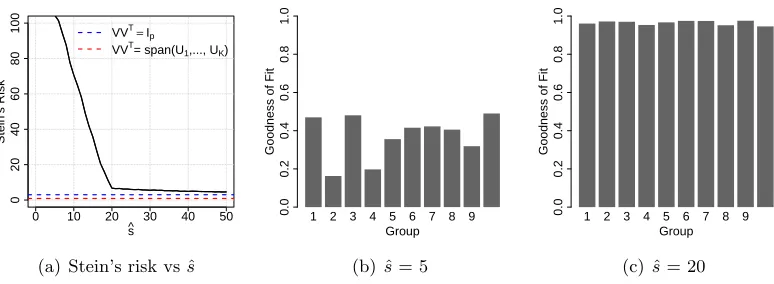
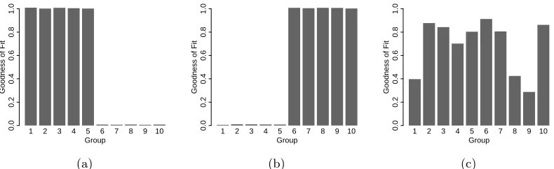
Figure 3: a) Stein’s risk as a function of the shared subspace dimension (solid black line). Data from ten groups, withUkgenerated uniformly on the Stiefel manifoldV200,2. As ˆs → p, the risk converges to the risk from independently estimated spiked covariance matrices (dashed blue line). The data also fit a shared subspace model with s = rK. If V VT = span(U1, ..., Uk) were known exactly, shared subspace
estimation yields lower risk than independent covariance estimation (dashed red line). b) For a single simulated data set, the goodness of fit statistic, γ(Yk :
ˆ
V ,σˆk2), when the assumed shared subspace is dimension ˆs= 5. c). For the same
data set, goodness of fit when the assumed shared subspace is dimension ˆs= 20. We can capture nearly all of the variability in each of the 10 groups using an ˆ
s=rK= 20 dimensional shared subspace.
We start by investigating the behavior of our model when we underestimate the true dimension of the shared subspace. In this simulation, we generateK= 10 groups of mean-zero normally distributed data withp= 200,r = 2,s=pandσk2= 1. We fix the eigenvalues of Ψk to (λ1, λ2) = (250,25). Although the signal variance from each group individually is preserved on a two dimensional subspace, these subspaces are not similar across groups since the eigenvectors from each group are generated uniformly from the Stiefel manifold,
Uk∈ Vp,r.
We use these data to evaluate how well the shared subspace estimator performs when we fit the data using a shared subspace model of dimension ˆs < s. In Figure 3(a) we plot Stein’s risk as a function of ˆs, estimating the risk empirically using ten independent simulations per value of ˆs. The dashed blue line corresponds to Stein’s risk for covariance matrices estimated independently. Independent covariance estimation is equivalent to shared subspace inference with ˆs= p because this implies V VT =Ip. Although the risk is large for small values of
ˆ
s, as the shared subspace dimension increases to the dimension of the feature space, that is ˆs → p, the risk for the shared subspace estimator quickly decreases. Importantly, it is always true that rank([U1, ..., UK])≤ rK so it can equivalently be assumed that the data
that is close to span([U1, ..., UK]). When ˆVVˆT = span([U1, ..., UK]) exactly, shared subspace
estimation outperforms independent covariance estimation (3(a), dashed red line).
From this simulation, it is clear that correctly specifying the dimension of the shared subspace is important for efficient covariance estimation. When the dimension of the shared subspace is too small, we accrue higher risk. The goodness of fit statistic,γ(Yk: ˆV ,σˆk2), can
be used to identify when a larger shared subspace is warranted. When ˆsis too small,γ(Yk:
ˆ
V ,σˆk2) will be substantially smaller than one for at least some of the groups, regardless
of ˆV (e.g. Figure 3(b)). When ˆs is large enough, we are able to use maximum marginal likelihood to identify a shared subspace which preserves most of the variation in the data for all groups (Figure 3(c)). Thus, for any estimated subspace, the goodness of fit statistic can be used to identify the groups that can be fairly compared on this subspace and whether we would benefit from fitting a model with a larger value of ˆs.
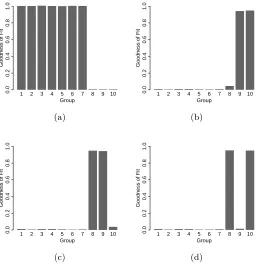
Finally, in the appendix, we include a some additional misspecification results. In par-ticular, we consider two cases in a 10 group analysis: one case in which 7 groups share a common subspace but the other three do not, and a second case in which five groups share one common two dimensional subspace, and the other five groups share a different two dimensional subspace (see Figures 8 and 9). Briefly, these results indicate that when only some of the groups share a common subspace, we can still usually identify both the existence of the subspace(s) shared by those groups. We can also identify which groups do not share the space, using the goodness of fit metric. When there are multiple relevant shared subspaces, we can often identify those distinct modes using a different subspace initialization for the EM algorithm.
Model Comparison and Rank Estimation: Clearly, correct specification for the rank
of the shared subspace is important for efficient inference. So far in this section, we have assumed that the group rank,r, and shared subspace dimension,s, are fixed and known. In practice this is not the case. Prior to fitting a model we should estimate these quantities. Standard model selection methods can be applied to select the both s and r. Common approaches include cross validation and information criteria like AIC and BIC. However, these approaches are computationally intensive since they require fitting the model for each value of s and r. Here, we estimate the model dimensions by applying an asymptotically optimal (in mean squared error) singular value threshold for low rank matrix recovery with noisy data (Gavish and Donoho, 2014). This rank estimator is a function of the median singular value of the data matrix and the ratio αk = p/nk. Note that under the shared
subspace model, the scaled and pooled data described in section 3.1 can be expressed as
Ypooled=X+Z whereV are the left singular values ofX andZ is a noise matrix with zero mean and variance one. This is the setting in which Gavish and Donoho (2014) develop a rank estimation algorithm, and so it can be appropriately applied toYpooled to estimates. Using this rank estimation approach, we conduct a simulation which demonstrates the relative performance of shared subspace group covariance estimation under different data generating models. We consider three different shared subspace data models: 1) a low dimensional shared subspace model with s=r; 2) a model in which the spiked covariance matrices from all groups are identical, e.g. Σk = Σ = UΛUT +σ2I; and 3) a full rank
Table 1: Stein’s risk (and 95% loss intervals) for different inferential models and data gen-erating models with varying degrees of between-group covariance similarity. For each of K = 10 groups, we simulate data from three different types of shared subspace models. For each of these models, p= 200, r = 2, σk2 = 1 and nk = 50.
We also fit the data using three different shared subspace models: a model in which s, r and V VT are all estimated from the data (“adaptive”), a spiked
co-variance model in which the coco-variance matrices from each group are assumed to be identical ( ˆΣk = ˆΣ) and a model in which we assume the data do not share a
lower dimensional subspace across groups (i.e. ˆs=p). The estimators which most closely match the data generating model have the lowest risk (diagonal) but the adaptive estimator performs well relative to the alternative misspecified model.
Inferential Model
Adaptive Σˆk= ˆΣ ˆs=p
Data
Mo
del s=r= 2 0.8 (0.7, 0.9) 2.1 (1.7, 2.6) 3.0 (2.9, 3.2) s=r= 2, Σk = Σ 0.8 (0.7, 0.9) 0.7 (0.6, 0.8) 3.0 (2.9, 3.2)
s=p= 200 7.1 (6.2, 8.0) 138.2 (119, 153) 3.0 (2.9, 3.2)
We estimate group-level covariance matrices from simulated data using three different variants of the shared subspace model. For each of these fits we estimate r. First, we estimate a single spiked covariance matrix from the pooled data and let ˆΣk = ˆΣ. Second,
we fit the full rank shared subspace model. This corresponds to a procedure in which we estimate each spiked covariance matrix independently, since s =p implies V VT = Ip.
Finally, we use an “adaptive” shared subspace estimator, in which we estimate both s, r
and V VT.
Since full rank estimators do not scale well, we compare the performance of various estimators on a simulated data set with only p = 200 features. We also assume forr = 2 spikes,σ2k= 1, and nk= 50. We fix the non-zero eigenvalues of Ψk to (λ1, λ2) = (250,25). We simulate 100 independent data sets for each data generating mechanisms. In Table 1 we report the average Stein’s risk and corresponding 95% loss intervals for the estimates derived from each of these inferential models.
As expected, the estimates with the lowest risk are derived from the inferential model that most closely match the data generating specifications. However, the adaptive estimator has small risk under model misspecification relative to the alternatives. For example, when Σk = Σ, the adaptive shared subspace estimator has almost four times smaller risk than
the full rank estimator, in which each covariance matrix is estimated independently. When the data come from a model in which s=p, that is, the eigenvectors of Ψk are generated
Finally, in addition to potential statistical efficiency gains, the empirical Bayes shared subspace estimator has significant computational advantages. In particular, the total run time for empirical Bayes inference of the shared subspace is significantly smaller than full Bayesian inference for a p×r dimensional subspace (e.g. Bayesian probabilistic PCA with
s = p), in particular for larger values of p. Given the difficulty of Bayesian inference on the Stiefel manifold, for largep, probabilistic principal component analysis quickly becomes infeasible. Empirical Bayes inference enables efficient optimization for ˆV and Bayesian inference on the lower dimensional shared subspace (See Figure 10, Appendix B, for typical run times).
5. Reduction of Asymptotic Bias Via Pooling
Recently, there has been an interest in the asymptotic behavior of PCA-based covariance estimators in the setting in which p, n→ ∞with p/n=α fixed. Specifically, in the spiked covariance model it is known that whenp and n are both large, the leading eigenvalues of the sample covariance matrix are positively biased and the empirical eigenvectors form a non-zero angle with the true eigenvectors (Baik and Silverstein, 2006; Paul, 2007). Although this fact also implies that the shared subspace estimators are biased, a major advantage of shared subspace inference over independent estimation of multiple covariance matrices is that we reduce the asymptotic bias, relative to independently estimated covariance matrices, by pooling information across groups. The bias reduction appears to be especially large when there is significant heterogeneity in the firstseigenvectors of the projected covariance matrices.
Throughout this section we assumeKgroups of data each withnk=nobservations per
group and sa fixed constant. First, note that if ˆVVˆT corresponds to the true shared sub-space, then estimates ˆψkderived using the methods presented in Section 3.2 will consistently
estimate ψk as n → ∞ regardless of whether p increases as well because YkV has a fixed
number of columns. For this reason, we focus explicitly on the accuracy of ˆVVˆT (derived using the maximum marginal likelihood algorithm presented in Section 3.1) as a function of the number of groupsK when both pand nare of the same order of magnitude and much larger thans. As an accuracy metric, we again study the behavior of tr( ˆVVˆTV VT)/swhich is bounded by zero and one and achieves a maximum of one if and only if ˆVVˆT corresponds
to the true shared subspace.
Conjecture 2 Assume that the firstseigenvalues from each ofK groups are identical with λi> σ2(1 +
√
α). Then, forp/n→α and p, n→ ∞, tr( ˆVVˆTV VT)/sa.s.→ ξ with
1> ξ ≥ 1
s
s
X
i=1
1− α
K(λi−1)2
/
1 + α
K(λi−1)
. (17)
We prove that the lower bound in 17 is in fact achieved when Yk are identically
dis-tributed and show in simulation that the subspace accuracy exceeds this bound when there is variation in the eigenvectors across groups. In the case of i.i.d. groups, let the covariance matrix Σk = Σ have the shared-subspace form given in Equation 2 and without loss of
eigenvectors of Σ). In this case, the complete data likelihood of V (Equation 5) can be rewritten as
`(V) = 1 2
X
k
tr
( 1
σ2I−M
−1)VTS
kV
= 1
2tr DV
T(X
k
Sk)V
!
.
wherePK
k=1Sk∼Wish(Σ, Kn). Sinceψis diagonal andσ2= 1,M =σ2(ψ+I) is diagonal and thusD= (σ12I−M
−1) is also diagonal with entries 0< d
i<1 of decreasing magnitude.
Then, the solution to
ˆ
V(k)= argmax
e
V∈Vp,s
tr DVeT X
k
(Sk)Ve !
.
has ˆV(k)equal to the first seigenvectors of P
kSk. This is maximized when the columns of
V match the first empirical eigenvectors ofP
kSk and has a maximum of
Pr
i=1di`i where
`i is the ith eigenvalue ofPkSk. Using a result from Paul (2007), it can be shown that as
long asλi > σ2(1 + √
α) where λi is theith eigenvalue of Σk, the asymptotic inner product
between the ith sample eigenvector and the ith population eigenvector approaches a limit that is almost surely less than one
|hVˆi, Vii| a.s.
→
s
1− α
K(λi−1)2
/
1 + α
K(λi−1)
As such, we can express asymptotic shared subspace accuracy for the identical groups model as
tr( ˆVVˆTV VT)/s= 1
s
s
X
i=1
|hVˆi, Vii|2
a.s. → 1
s
s
X
i=1
1− α
K(λi−1)2
/
1 + α
K(λi−1)
. (18)
Here, the accuracy of the estimate depends onα,K and the magnitude of the eigenval-ues, with the bias naturally decreasing as the number of groups increases. Most importantly, Equation 18 provides a useful benchmark for understanding the bias of shared subspace es-timates in the general setting in which ψk varies across groups. Our conjecture that the
subspace accuracy is larger than the lower bound when the eigenvectors between groups are variable is consistent with our simulation results.
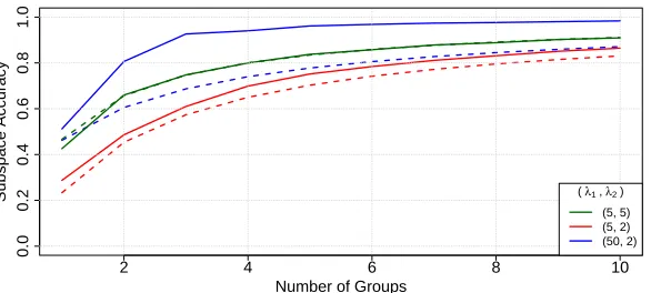
In Figure 4 we depict the subspace accuracy metric tr( ˆVVˆTV VT)/s and benchmark 1
s
Ps
i=1
1−K(λα
i−1)2
/
1 +K(λα
i−1)
for simulated multi-group data generated under the shared subspace model with s= 2, n= 50, p= 200 and three different sets of eigenvalues. For each covariance matrix, the eigenvectors ofψkwere sampled uniformly from Stiefel
2 4 6 8 10
0.0
0.2
0.4
0.6
0.8
1.0
Number of Groups
Subspace Accur
acy
( λ1 , λ2 ) (5, 5) (5, 2) (50, 2)
Figure 4: Subspace accuracy tr( ˆVVˆTV VT)/s(solid) and the asymptotics-based benchmark (dashed) as a function of K. When λ1 = λ2 (green), the assumptions used to derive the benchmark (identically distributed groups) are met and thus the subspace accuracy matches the benchmark. However, when the ratio λ1/λ2 is large, the subspace accuracy metric can far exceed this benchmark if there is significant variation in the eigenvectors of ψk across groups. Small increases in
accuracy over the benchmark are seen for moderately anisotropic data (red) and large increases for highly anisotropic data (blue).
benchmark since the assumptions used to derive this asymptotic result are met. However, when the eigenvectors of ψk vary significantly across groups and λ1 λ2, the subspace accuracy can far exceed this benchmark (blue). Intuitively, when the first eigenvectors of two different groups are nearly orthogonal, each group provides a lot of information about orthogonal directions on V VT and so the gains in accuracy exceed those that you would get by estimating the subspace from a single group with K times the sample size. In gen-eral the accuracy of shared subspace estimates depends on the variation in the eigenvectors of ψk across groups as well as the magnitude of the eigenvalues and matrix dimensions p
and nk. Although the shared subspace estimator improves on the accuracy of individually
estimated covariance matrices, estimates can still be biased when α is very large or the eigenvalues of Σk are very small for allk. In practice, one should estimate the approximate
magnitude of the bias using the inferred eigenvalues of Σk. When these inferred eigenvalues
are significantly larger than ˆσk2(1 +pα/K) the bias will likely be small.
6. Analysis of Gene Expression Data
on mean level differences between expression levels. In particular, mean-level differences can be useful for identifying leukemia subtypes. However, differences in the covariance struc-ture across groups can be induced by interactions between important unobserved variables. Covariance analysis is particularly important when the effects of unobserved variables, like disease severity, disease progression or unmeasured genetic confounders, dominate mean level differences across groups. In this analysis, we explicitly remove the mean from the data and look for differences in the covariance structure of the gene expression levels.
The data we analyze were generated from 327 bone marrow samples analyzed on an Affymetrix oligonucleotide microarray with over 12,000 probe sets. Preliminary analysis using mean differences identified clusters corresponding to distinct leukemia subtypes: BCR-ABL, E2A-PBX1, hyperdiploid, MLL, T-ALL, TEL-AML1. 79 patients were assigned to a seventh group for unidentified subtypes (“Others”). We use these labels to stratify the obser-vations into seven groups with corresponding sample sizes of n= (15,27,64,20,43,79,79). Although there are over 12,000 probes on the microarray, the vast majority of gene expression levels are missing. Thus, we restrict our attention to the genes for which less than half of the values are missing and use Amelia, a software package for missing value imputation, to fill in the remaining missing values (Honaker et al., 2011). Amelia assumes the data is missing at random and that each group is normally distributed with a common covariance matrix. Since imputation is done under the assumption of covariance homogene-ity, any inferred differences between groups are unlikely to be an artifact of the imputation process. We leave it to future work to incorporate missing data imputation into the shared subspace inference algorithm. After removing genes with very high percentages of missing values, p= 3124 genes remain. Prior to analysis, we de-mean both the rows and columns of the gene expression levels in each group.
We apply the rank selection criteria discussed in Section 4.1 and proposed by Gavish and Donoho (2014) to the pooled expression data (i.e. data from all groups combined) to decide on an appropriate value for the shared subspace. This procedure yields s = 45 dimensions1. We run Algorithm 1 to estimate the shared subspace, and then use Bayesian inference (Algorithm 2) to identify differences between groups on the inferred subspace. Together, the run time for the full empirical Bayes procedure (both algorithms) took less than 10 minutes on a 2017 Macbook Pro.
Using the goodness of fit metric, we find that a 45-dimensional shared subspace di-mension that explains over 90% of the estimated variation in the top s eigenvectors of Σk, suggesting that the rank selection procedure worked reasonably well (Figure 11(a),
Appendix B). To further validate the utility of shared subspace modeling, we look at how informative the projected data covariance matrices are for predicting group mem-bership. For an observation Yi, we compute the probability, assuming uniform prior
dis-tribution over group membership, that Yi came from group k as P(Yi from groupk) =
|Ψk|−1/2etr(−1/2(YiVˆ)TΨ−k1YiVˆ)
P
j(|Ψj|−1/2etr(−1/2(YiVˆ)TΨ−j1YiVˆ)). We correctly identified the leukemia type in all samples,
which provides further confirmation that this subspace provides enough predictive power to easily distinguish groups.
In addition, we quantified differences amongst the projected data covariances using the Frobenius norm,||Ψk−Ψj||F for all pairs of the seven groups. We use these distances to
pute a hierarchical clustering dendrogram of the groups (Figure 11(b), Appendix B). The hierarchical clustering reveals that BCR-ABL, E2A-PBX1, TEL-AML1 and hyperdiploid, which correspond to B lineage leukemias, cluster together. T-ALL, the T lineage leukemia, and MLL, the mixed lineage leukemia, appear the most different (Dang, 2012). To further verify that the inferred subspace relates to relevant biological processes, we conducted gene set enrichment analysis using the observed magnitudes of the loadings for the genes on the 45 basis vectors (Subramanian et al., 2005) and using gene sets defined by the Gene On-tology Consortium (Consortium et al., 2004). Gene set analysis on the magnitudes of gene loadings identified dozens of pathways (FDR < 0.01, (Storey et al., 2003)). Nearly every identified pathway relates to the immune response or cell growth (Figure 12, Appendix B), for example B and T cell proliferation (GO:0042100, GO:0042102), immunoglobin receptor binding (GO:0034987) and cellular response to cytokine stimulus (GO:0071345) to name only a few. Together, all of these results suggest that in this application there is indeed significant differences in the covariability between genes for each the of groups, with bio-logically plausible underpinnings. Consequently, there is value in exploring what underlies those differences.
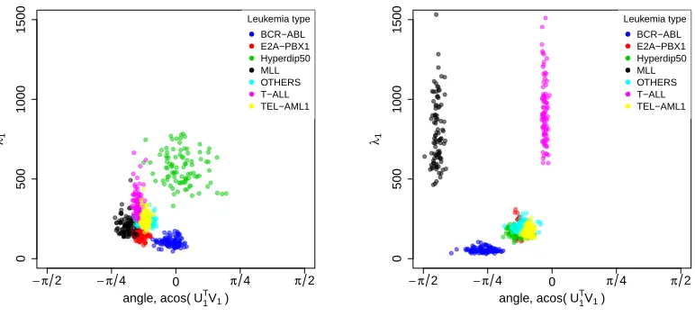
We next demonstrate how we can explore significant a posteriori differences between the groups which might lead to scientifically meaningful insights. In order to visualize differences in the posterior distributions of the 45×45 dimensional matrices Ψk, we examine
the distribution of eigenvalues and eigenvectors between the groups on a variety of two-dimensional subspaces of the shared space. We propose two different methods for identifying potentially interesting sub-subspaces to visualize. First, we summarize variation on a two dimensional subspace whose axes are approximately aligned to the first two eigenvectors of
ˆ
Σk, for a specific groupk. This subspace corresponds to the subspace of maximal variability
within groupk. For example, in Figure 5(a) we plot posterior summaries about the principal eigenvector and eigenvalues for each group on a two dimensional space spanned by the first two eigenvectors of the inferred covariance matrix for the hyperdiploid group. The x -axis corresponds to the orientation of the first eigenvector and the y--axis corresponds the magnitude of the first eigenvalue. In this subspace, we can see that the first eigenvector for most groups appear to have similar orientations, but that the hyperdiploid group has significantly larger variance along the first principal component direction than all other groups (with the exception of perhaps T-ALL, for which the posterior samples overlap). The first eigenvector for the BCR-ABL subgroup appears to be the least variable on this subspace.
As an alternative approach to summarizing the posterior distribution, we examine the posterior eigen-summaries on a two dimensional subspace which is chosen to maximize the difference between any two chosen groups. To achieve this, we look at spaces in which the axes correspond to the first two eigenvectors of ˆΣk−Σˆj for any k 6= j. As an example,
0
500
1000
1500
angle, acos(U1
T
V1)
λ1
− π 2 − π4 0 π4 π2
●
●
●
●
●
●
●
Leukemia type
BCR−ABL E2A−PBX1 Hyperdip50 MLL OTHERS T−ALL TEL−AML1
(a) Subspace for hyperdiploid subtype
0
500
1000
1500
angle, acos(U1
T
V1)
λ1
− π2 − π 4 0 π4 π2
●
●
●
●
●
●
●
Leukemia type
BCR−ABL E2A−PBX1 Hyperdip50 MLL OTHERS T−ALL TEL−AML1
(b) T-ALL vs MLL subspace
Figure 5: Posterior samples for the first eigenvalue and orientation of the first eigenvector on the a dimensional subspace. a) The two dimensional subspace was chosen to approximately span the first two eigenvectors for the hyperdiploid group. The orientation of first eigenvector is similar for all groups, but the variance signifi-cantly larger for the hyperdiploid subgroup. b) The two dimensional subspace was chosen to maximize the difference between the T-ALL and MLL groups. Along the first dimension of this subspace, there is large variability in the T-ALL group that is not matched in other groups, whereas the second dimension there is large variability in the MLL group that is not matched in the other groups.
Scientific insights underlying the significant differences that were identified in Figure 5 can be understood in the biplots in Figures 6 and 7. In each figure, we plot the contours of the two dimensional covariance matrices for a few leukemia subtypes. The 20 genes with the largest loadings for one of the component directions are indicated with letters and the remaining loadings plotted with light grey dots. The gene names for the genes with the largest loadings are listed in the corresponding table. In both biplots, the identified genes have known connections to cancer, leukemia, and the immune system.
For example, for the subspace of maximal variability in the hyperdiploid group, gene set analysis identified two gene sets with large magnitude loadings on the first principal component: a small group of proteins corresponding to the MHC class II protein complex (GO:0006955) as well as a larger group of genes corresponding to genes generally involved in immune response (GO:0006955). MHC class II proteins are known to play an essential role in the adaptive immune system (Reith et al., 2005) and are correlated with leukemia patient outcomes (Rimsza et al., 2004). Our analysis indicates these proteins have especially variable levels in the hyperdiploid subtype relative to the other leukemia subtypes.