MURDOCH RESEARCH REPOSITORY
http://dx.doi.org/10.1109/42.640738
Chandrasekhar, R. and Attikiouzel, Y. (1997) A simple method
for automatically locating the nipple on mammograms. IEEE
Transactions on Medical Imaging, 16 (5). pp. 483-494.
http://researchrepository.murdoch.edu.au/18456/
Copyright © 1996 IEEE
Personal use of this material is permitted. However, permission to reprint/republish
this material for advertising or promotional purposes or for creating new collective
A Simple Method for Automatically Locating
the Nipple on Mammograms
Ramachandran Chandrasekhar,*
Member, IEEE, and Yianni Attikiouzel,
Fellow, IEEEAbstract— This paper outlines a simple, fast, and accurate
method for automatically locating the nipple on digitized mam-mograms that have been segmented to reveal the skair in-terface. If the average gradient of the intensity is computed in the direction normal to the interface and directed inside the breast, it is found that there is a sudden and distinct change in this parameter close to the nipple. A nipple in profile is located between two successive maxima of this parameter; otherwise, it is near the global maximum. Specifically, the nipple is located midway between a successive maximum and minimum of the derivative of the average intensity gradient; these being local turning points for a nipple in profile and global otherwise. The method has been tested on 24 images, including both oblique and cranio-caudal views, from two digital mammogram databases. For 23 of the images (96%), the rms error was less than 1 mm at image resolutions of 400m and 420 m per pixel. Because of its simplicity, and because it is based both on the observed behavior of mammographic tissue intensities and on geometry, this method has the potential to become a generic method for locating the nipple on mammograms.
Index Terms—Automatic nipple location, computer vision,
im-age processing, mammograms.
I. INTRODUCTION
M
AMMOGRAMS are X-ray images of the breast. At present, they are the method of choice for screening asymptomatic women for early detection of breast cancer. Such screening will necessarily generate a large number of mammograms which must be viewed and interpreted by a limited number of expert radiologists. Automatic analysis of mammograms by computer, as the first stage in analyzing mammograms, could serve to reduce the workload on radi-ologists.Before mammograms can be analyzed by machine, they must be digitized with adequate greyscale and spatial reso-lution. It is also vital to ensure that low-intensity features such as the skin-air interface and the nipple are preserved
Manuscript received August 10, 1995; revised May 16, 1997. The work of R. Chandrasekhar was supported by an Australian Overseas Postgraduate Re-search Scholarship (OPRS) from the Australian Commonwealth Government and a University Research Studentship (URS) from the University of Western Australia. The Associate Editor responsible for coordinating the review of this paper and recommending its publication was C. Roux. Asterisk indicates corresponding author.
*R Chandrasekhar was with the Center for Intelligent Information Pro-cessing Systems, Department of Electrical and Electronic Engineering, The University of Western Australia, Nedlands, WA 6907, Australia. He is now with the Biomedical Engineering Department, Singapore General Hospital, Singapore 169608 Singapore (e-mail: [email protected]).
Y. Attikiouzel is with the Center for Intelligent Information Processing Systems, Department of Electrical and Electronic Engineering, The University of Western Australia, Nedlands, WA 6907, Australia.
Publisher Item Identifier S 0278-0062(97)07789-6.
with fidelity during digitization. Assuming that this has been done, the first stage of preprocessing is segmentation of the image into background and object. This should yield a clear and smooth skin-air interface.
The next logical step would be to locate the nipple on the mammogram. There are several reasons why this should be done. Anatomically, the nipple is the only landmark on the breast [1, p. 119]. The glandular structures comprising the lobules, ductules, lobes, and ducts hierarchically converge onto the nipple. Because cancer arises in the glandular tissue of the breast [1, p. 121], it would be sensible for any automatic search strategy for detecting cancer to begin at the nipple and fan out into the “cone” or “triangle” of glandular tissue that has the nipple as its apex. Moreover, given its singularity, radiologists pay specific attention to the nipple as part of their examination of a mammogram [2, p. 22], [3, p. 123]. Radiologists also compare corresponding regions of the right and left breasts to detect relative anomalies [2, p. 22]. Computer methods that attempt the same task rely heavily on the nipple as an alignment pivot [4], [5].
This paper reports on a simple method for locating the nipple on a mammogram. It has been tested on a total of 24 images. Sixteen of these are oblique-view mammograms from a digital database made available to researchers by the Mammographic Image Analysis Society (MIAS) of the United Kingdom [6], [7]. The remaining eight images are cranio-caudal views from another database of digitized mammograms distributed by the University of California, San Francisco, CA (UCSF), and the Lawrence Livermore National Laboratory (LLNL), Livermore, CA [8]. These two databases shall hence-forth be referred to by the acronyms MIAS and UCSF/LLNL, respectively.
II. REVIEW OF PREVIOUS WORK
There are relatively few reports in the literature on automatic nipple location. The problem was first discussed by Semmlow
et al. [9] in their paper on the automated screening of
xe-romammograms. They used a special shape-sensitive spatial filter to generate measures of roughness and directionality to locate the central region of the breast boundary. The lowest point on this boundary was then taken to be the nipple—a debatable geometric assumption. A more recent1 account of
automatic nipple location is that by Yin et al. [5], reported
1While the present paper was under review, Mendez et al. [10] published a paper on automatic detection of the breast border and nipple. Their work was motivated by observations similar to ours, although the nipple detection method described therein is different from that presented here. Interested readers are referred to the original paper for details.
(a) (b) (c)
Fig. 1. Effect of ramping the intensities on MIAS mammogram 003. (a) Original byte-image mammogram. (b) Eight-cycle ramp obtained by setting
In = 8Iomod 256: (c) Sixty-four cycle ramp clearly outlining the nipple, whose intensity does not vary much. Note also that the lower background
is markedly nonuniform.
as part of a bilateral-subtraction technique to detect masses in mammograms. They extracted the breast border and averaged the grey values in small 10 by 40 pixel regions for points along the border. They then plotted the relative average intensity value against location along the border and identified the nip-ple at the location of the maximum on the plot. They reported that for images digitized at 400 m per pixel, the nipple position found by computer differed on average by 10 mm from that located by a radiologist. In their study, no mention was made of whether or not the nipple was in profile in any of the segmented images, but we believe that their method would fail for a mammogram in which the nipple is in profile.
III. OUTLINE OF METHOD
The method we describe here is based principally on the observed behavior of the pattern of intensities on the mam-mogram adjacent to the skin-air interface. It was observed that the iso-intensity contours there follow the direction of the skin-air interface and run more or less parallel to it. Near the region of the nipple, however, the iso-intensity contours slope rather sharply toward the skin-air interface. A form of intensity
aliasing may be used to demonstrate this. For example, on a
byte image where each pixel may take a value from 0–255, an cycle intensity ramp may be applied to each original intensity value, , to yield the new intensity, given by
(1)
where stands for the remainder when is divided by , both and being integers. Fig. 1 shows an original mammogram and the images obtained by ramping the inten-sities for eight and 64 cycles, to better display low-intensity levels. It is clear from Fig. 1(b) that the iso-intensity contours
are more closely packed as they slope toward the nipple.
If the nipple appears in profile on the mammogram, the
intensity of the nipple is always comparatively low and varies little in the region of the protuberance. This is most easily
seen by displaying the mammogram in color using a random
colormap. It may also be seen by intensity-ramping the image as shown in Fig. 1(c). Note also the marked nonuniformity of the background made apparent in this image although not obvious in the original.
Based on these two observations, we framed the following hypothesis.
1) The nipple is located on the mammogram close to where the intensity gradient in the direction normal to the skin-air interface and directed inside the breast is a maximum. 2) In cases where the nipple is in profile, its relatively unchanging, low intensities mean that it would be lo-cated close to a minimum of the intensity gradient in the normal direction.
Two assumptions underlie this hypothesis.
1) The nipple, whether in profile or not, is situated on or very close to the skin-air interface.
2) The nipple points in the direction of the normal to the skin-air interface.
Experiments were performed on 24 mammograms from two databases to ascertain whether this hypothesis was justified, and if so, whether it could be used to locate the nipple reliably on a mammogram.
IV. NOTATION
The image is treated as a discrete-valued function,
of two integer variables, and with the origin at the top left-hand corner of the image, orientated as shown in Figs. 1(a) and 2. This means that the value runs positive from top to bottom, anomalously. Because the breast sometimes can and does curve in on itself in the oblique-view, the value is used to index position rather than the value. We will denote the original image as The number of pixels in the image in the - and -directions are denoted by and , respectively. The resolution of the image in both the - and
-directions is mm per pixel.
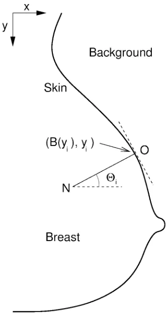
Fig. 2. The breast is orientated so that the nipple always faces the right. The coordinate axes are directed as shown with the origin corresponding to the top left corner of the image. The normal to the breast at the point(B(yi); yi) on
the skin-air interface is directed breastwards in the directionON as shown. The intensity gradient along the normal is computed using the pixels lying onON: The angle 2imade by the normal with the positivex-direction is also shown.
intensity gradient is used, it connotes the rate of change of
intensity with Euclidean distance in a particular direction on the - plane.
V. DETAILED DESCRIPTION OFALGORITHM
The detailed description of the algorithm is given below. 1) The breast is segmented from the background, either
in-teractively (semiautomatically) or automatically, special care being taken to preserve with fidelity as much as possible of the breast portion of the skin-air interface, including the nipple, if it is in profile. Because of the variation in the background, [see Fig. 1(c)], and the possibility that the same intensity could represent breast tissue in one region of the image and background in another, simple thresholding would not necessarily work always. Another precaution is to ensure that the extracted skin-air interface is smooth to the eye at the resolution of the image. This results in a labeled binary image, , showing the breast and background [see Fig. 3(b)].
2) The border of the breast, representing the skair in-terface, is extracted from the labeled image. We denote
this by , defined for all integer values of running from 0 to gives the value of the skin-air boundary for a given Implicit in this is the assumption that is well defined. This may not hold at the inferior portion of the breast, near the infra-mammary crease and the chest wall, but those regions will usually be excluded from our search as explained below. 3) We restrict the search for the nipple to values of
lying between and For convenience, these values of will be denoted by and , respectively, the general value lying within these limits being denoted by This restriction avoids unnecessary computation as well as edge artifacts (such as tapes) that sometimes appear at the edges of the digitized images. It also circumvents problems arising from not being well defined in the inferior portion of the breast. A similar restriction is also imposed on the allowable values by requiring to be greater than , again to avoid edge effects and artifacts such as skin folds.
4) For each of the test points, , on , we estimate the tangent to by the straight line that best fits (in the sense of least squared error) a neighborhood of points on the border, centered on The gradient of this line is denoted by
5) The gradient (and hence direction) of the normal at is estimated as taking into account the anomalous coordinate system described above. As-sociated with this normal is the angle that it makes with the positive -direction (see Fig. 2).
6) Pixels lying on the normal at various integer distances from the test point are identified, and for each of these, , the intensity
gradient along the normal direction is computed simply
as
for and (2)
We call the depth of the normal. The average of these intensity gradients is defined to be the average intensity
gradient along the normal,
for (3)
7) The sequence is smoothed by a smoothing filter , and the resulting sequence is normalized to yield the zero mean, unit variance sequence, This latter sequence is passed through a differentiator , to yield
Likewise, is smoothed and normalized to yield and differentiated to give
9) The maximum value of is then found. It is denoted by and its index by The minimum value of , is also found and its position denoted by
10) If is less than a predefined negative threshold , the nipple is inferred to be in profile; otherwise, it is not. Because the vary across a predictable range of values in all images, it was possible to use an absolute threshold on without sacrificing generality. (Occasionally, because of poor segmentation or an image with an uneven skin-air interface, the value of could lie below the threshold even when the nipple is not in profile. To exclude such cases, we check to see if the indexes and lie within a certain distance of each other, called the nipple window If they do, the nipple is in profile; otherwise it is not.) 11) The algorithm automatically bifurcates here depending
on whether or not the nipple is in profile (as determined above)
a) Nipple is not in profile: The indexes of the global maximum, , and minimum, , of the derivative curve are located and denoted by and , respectively. The value of the computed nipple position is given by where
(4)
and the nipple position is then One comment is in order here: we have found that is often a good first estimate for Therefore, if the global maximum and minimum lie within one nipple
window of , the estimate may be considered more reliable than otherwise. Although this reliabil-ity measure is not used in these results, through its use, the algorithm may itself estimate the reliability of its nipple detection and pass that information on to other program segments, in the context of a more ambitious automatic global segmentation of mammograms. It could also be used to improve the performance of this algorithm adaptively.
b) Nipple is in profile: The local minimum on imme-diately preceding is found. Let us call it and its position The local maximum, , that occurs immediately after is then found and its position, , ascertained. The value of the computed nipple position is given by where
(5)
and the nipple position is again
VI. EXPERIMENTAL METHOD
A. Preliminary
Our algorithm was developed and tested using oblique-view images from the MIAS database. However, since that database lacks cranio-caudal views, we subsequently used images from the UCSF/LLNL database to test our method on cranio-caudal views as well. The images in the two different databases were
acquired and presented differently. Accordingly they were preprocessed differently.
The MIAS images are distributed as 8-bit-per-pixel greyscale images at 50 m per pixel spatial resolution in each orthogonal direction. The images were simultaneously shrunk and lowpass filtered by averaging within an 8 8 window and assigning the result to the new pixel value. The resolution of the test images was, therefore, 400 m per pixel in each direction. It is noteworthy that pixel values in the MIAS database were assigned using a detector that was linear
in the optical density (O.D.) range of 0 to 3.2 [6], [7].
The UCSF/LLNL images are distributed as 12-bit-per-pixel greyscale images at 35 m per pixel in each orthogonal direction. These images were likewise averaged and shrunk within a 12 12 window to yield working images having a resolution of 420 m per pixel in each direction. We note however, that during digitization, the pixel values for the UCSF/LLNL database were assigned linearly with transmitted
intensity [11] (rather than optical density as in the MIAS
database). To test images from this database on the same software, the 12-bit images were transformed into 8-bit-per-pixel images by retaining the 256 lowest levels in each image and clipping all higher pixel values to 255. We felt justified in doing this since we were concerned with the low-intensity end of the image in our algorithm.
The method was tested on 16 oblique-view images from the first 80 in the MIAS database. The images were selected to include cases where the nipple was in profile and where it was not. The latter category included three images where the nipple was noticeably recessed. Eleven of the fifteen test cases were normal mammograms which ranged from fatty to glandular to dense, as classified by the MIAS. Of the remaining five, two exhibited benign changes and three were malignant.
The algorithm was also tested on 18 cranio-caudal images from the UCSF/LLNL database. These images were not se-lected by us, but had been used by other researchers working on a different project. We report on the results for eight of the images here. The results for some of the remaining images were not as good and point to the need for additional preprocessing—a subject that we have dealt with elsewhere [12], because it raises larger issues such as the effect of method of digitization on algorithm performance across databases.
All images used for these experiments were rotated so that the nipple always faced the right, whether of a right- or left-breast mammogram. The labeled binary image, , was generated by modeling the image background as a polyno-mial, subtracting it out, thresholding the subtracted image and region-filling the resulting image to obtain a smooth, contiguous border. This step was semiautomatic, with the user selecting two parameters interactively for the MIAS images, and entirely automatic for the UCSF/LLNL images. The details of this preprocessing are beyond the scope of this paper and have been described in full elsewhere [12], [13].
B. Choice of Parameter Values
TABLE I
VALUESASSIGNED TO THEDIFFERENTPARAMETERSUSED IN THEALGORITHM ANDTHEIRMEANINGS
Symbol Value Description
r varies Resolution of image in mm per pixel in either direction.
ny varies Length of image in pixels iny direction.
y1
yn
0:3ny
0:95ny
The search for the nipple is restricted to values ofy lying between y1andyn:
p 10=r Number of points in the neighborhood of each test point used to estimate the tangent at that point. Set to the number of pixels in 10 mm.
k 10=r Depth to which intensity gradients along the normal are computed before being averaged. Set to the number of pixels in 10 mm.
l 10=r Length of smoothing and derivative filters. Set to the number of pixels in 10 mm.
t 00:4 The absolute threshold against which the minimum value of0iis tested. If0min< t the nipple could be in profile; not otherwise. If0is scaled by 5, the test becomes
0
min< 02:0:
w 20=r Length of nipple window within which bothgmaxandmin0 should lie if the nipple is in profile. Set to the number of pixels in 20 mm.
characteristic dimensions. It was decided, therefore, to express parameters in terms of such dimensions wherever possible. For example, the “diameter” of the nipple in profile was taken to be typically 10 mm (based on preliminary experiments with the MIAS database) and this value was used to determine the lengths of the smoothing and derivative filters. By expressing the filter length of 10 mm in terms of the pixel-resolution of the image in mm per pixel, this value was automatically scaled with the image. To avoid dependence on “magic numbers” and give the method generality, we have expressed most parameters in terms of or in terms of , the length of the image, which is inversely proportional to These values are shown in Table I.
C. Filters
A raised cosine smoothing filter was chosen because it was analytic, differentiable, had compact support, and was zero at both extremes. The sine filter used to differentiate the smoothed data was chosen because it was analytically the derivative of the smoothing filter. Both filters were normalized so that the sum of the absolute values of their coefficients was unity. The sine filter functions as a smoothing filter for half its length and, thereby, distorts the derivative values at either end of the input sequence. For this reason, the number of data points at the beginning and end, equal to the filter length, were discarded from the derivative data. As explained earlier, the filter lengths themselves were chosen to match the size of the structure being detected, namely the nipple. The derivative data were scaled five times to occupy a similar range as the smoothed data.
D. Effect of Varying Parameters
The method was tested out on MIAS images at resolutions of 800 m per pixel and 1200 m per pixel and found to yield results consistent with those from the images at 400 m per pixel.
The depth parameter was also varied. In cases where the nipple was in profile, could be varied from about 5 mm (i.e., to 10 mm, to yield consistent results; varying it above 10 mm led to the normal transecting the nipple and going
beyond the extent of the object region in However, in cases where the nipple was not in profile, and especially in the case of image 051 (discussed below) where the nipple is recessed from the skin-air interface by a distance greater than increasing gave results of similar accuracy to the other images.
E. Reference Data
The position of the nipple was manually identified by a ra-diologist using a mouse and thexvInteractive Image Display program (version 3.10a) [14]. The Sun display terminal used was 1152 900 pixels at 83 82 dots per inch. The MIAS images at 400 m per pixel, and the UCSF/LLNL images at 420 m per pixel were used for this purpose.
The reference data and the results of the experiments are given in Table II. The positions of the superior/inferior or medial/lateral extents of the nipple were identified by the radiologist; the coordinates of these positions were used as the range values. The radiologist also identified the
position of the nipple on the skin-air interface three times and the average of these values gave the value in Table II.
In three images, the nipple was noticeably recessed from the skin-air interface. In these cases, the actual nipple position was different from the three values on the skin-air interface used to obtain the values. These images are considered in more detail later.
VII. RESULTS AND DISCUSSION
The test mammograms fell into two main classes: 1) nipple fully or partly in profile;
2) nipple not in profile.
In Table II, the column labeled gives the computer-detected nipple location in accordance with (4) or (5). The column labeled gives the error in pixels between , the computer-identified position, and the reference nipple position, The column headed by gives the values of the
midpoint of the positions of the global maximum and minimum
TABLE II
RESULTS OFAUTOMATICNIPPLEDETECTION ON16 OBLIQUE-VIEWMAMMOGRAMS FROM THE MIAS DATABASE(NUMBEREDIMAGES)ANDEIGHTCRANIO-CAUDAL-VIEW MAMMOGRAMS FROM THEUCSF/LLNL DATABASE(LETTEREDIMAGES). SEETEXT
FOREXPLANATION OFCOLUMNHEADINGS ANDDISCUSSION
Image
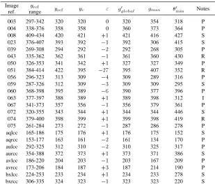
ref. rangeyref yref yc " g0global gmax min0 Notes
003 297-342 320 320 0 320 354 318 P
004 338-376 358 358 0 360 373 364 P
008 409-434 420 421 +1 421 416 427 S
023 376-407 393 392 01 392 306 415 S
039 269-308 294 292 02 292 268 305 P
043 335-362 362 361 01 361 360 430 R
050 326-353 341 342 +1 327 327 349 P
051 384-414 422 395 027 395 407 352 R
056 296-323 313 309 04 309 289 316 P
059 287-326 312 309 03 309 309 295 S
060 368-398 395 389 06 390 377 396 P
063 377-397 388 389 +1 389 398 312 I
067 341-373 357 356 01 356 379 361 P
072 320-355 343 344 +1 344 344 446 S
074 379-400 398 399 +1 399 398 419 R
075 261-284 273 272 01 287 286 278 P
aqlcc 165-186 175 176 +1 176 175 152 S
aqrcc 153-177 163 161 02 161 134 170 P
aulcc 292-325 312 310 02 310 325 317 P
aurcc 354-388 372 373 +1 373 371 386 S
avlcc 186-220 204 203 01 203 167 209 P
avrcc 173-206 184 187 +3 187 214 190 P
bxlcc 224-253 233 234 +1 234 233 278 S
bxrcc 306-335 324 323 01 323 323 220 S
the following: P: nipple fully or partly in profile; S: nipple not in profile, but close to or at the skin-air interface; R: nipple noticeably recessed from skin-air interface; I: inverted nipple.
A. Nipple in Profile
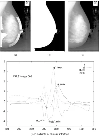
A nipple in profile is seen in MIAS image 003, illustrated in Fig. 3. The labeled image is shown in Fig. 3(b) where the skin-air interface is defined by the white border adjacent to the black region. This border is used to estimate the tangent and normal directions at every value on the border between and The normals are shown drawn on Fig. 3(a). The average value of the intensity gradient along the normal is plotted against the coordinate at the left of Fig. 3(a). Note the clear dip in the average intensity gradient at values close to where the nipple is. This behavior is characteristic of the nipple in profile and results from the normals traversing tissue corresponding to the protruding nipple, which we have observed is an almost uniform, low-intensity region on the mammogram. However, the absolute magnitudes of the minimum and the two maxima that abut it vary across images, precluding thresholding of as a reliable feature.
Fig. 3(d) shows the smoothed plots of and The trough in the - curve corresponding to the nipple occurs for values between 300 and 350. Note also the rapid change in the - curve for this same range of values. Because the nipple in profile is at most a semicircular protuberance, this change is bounded: at most, it is of the order of across a region that is about 10 mm. In other words, we
may justifiably set an absolute threshold for to detect the
nipple in profile, which is what we do. However, although
is a well-behaved parameter, it tends to over estimate the position of the nipple as shown in Table II. This is because, is a geometric parameter that is affected by the orientation of the nipple in profile. A characteristic based on tissue intensity will not suffer this drawback. If we use the position of as an anchor, we observed that there was always a local
minimum of preceding the minimum of This is and the local maximum following it is The nipple was always located between the positions defined by and We have consistently found that for our test images,
the nipple position may be estimated reliably and accurately by the midpoint between the positions of and We note in passing that these two turning points define the two steep drops in that enclose the trough, i.e., their midpoint roughly indicates the middle of the trough corresponding to the nipple.
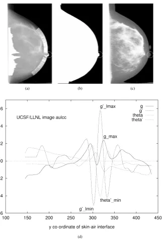
The results for cranio-caudal images from the UCSF/LLNL database follow the same pattern as for the oblique-view mammograms from the MIAS database. An example is shown in Fig. 4. Note that although the trough on the - curve corresponding to the nipple in profile is not as pronounced in this case as in Fig. 3(d), the average of the positions of and again gives a good estimate of the nipple position.
B. Nipple Not in Profile
(a) (b) (c)
(d)
Fig. 3. MIAS image 003 in oblique view with nipple clearly in profile. (a) The intensities on the original mammogram have been histogram-equalized. (b) Labeled image showing skin-air interface. (c) The estimated nipple position is at the center of the circle and corresponds to ay value of 320; the radiologist-determined reference nipple position is aty = 320: (d) Graphs of normal intensity gradient g, its derivative g0, the angle, and its derivative 0 plotted againsty coordinate of skin-air interface. The center of the circled nipple position is the y value lying midway between the positions of gl min0 andg0l max:
may be grossly estimated by the position of Indeed, in this case, the midpoint of the positions of and , the global maximum and minimum, respectively, of , equals the position of at , which again is close to the reference position at We have chosen to use the midpoint of and in preference to because the former better reflects the rapid change in the intensity gradient associated with the nipple. The maximum, being a single value, may or may not be located symmetrically about these rapid changes in intensity gradient. The results in Table II bear this out for the images tested. Note that the position of is not relevant here, and in any case,
Even if the nipple is in profile in the original image, if the labeled image is the result of over-thresholding (i.e., the boundary on represents not the skin-air interface, but rather some interface between tissues in the breast) the plot of
etc., will be similar to Fig. 5(d).
It is noteworthy that the maximum we are dealing with here is the maximum of the average intensity gradient in the direction normal to the skin-air interface, whereas the maximum used by Yin et al. [5] is the maximum of the average
intensity directed along the border.
(a) (b) (c)
(d)
Fig. 4. UCSF/LLNL image aulcc in cranio-caudal view with nipple clearly in profile. (a) The intensities on the original mammogram have been transformed logarithmically for display. (b) Labeled image showing skin-air interface. (c) This image has been histogram-equalized for display. Note the background “noise” above the nipple which was subtracted out by preprocessing. The estimated nipple position is at the center of the circle and corresponds to ay value of 310; the radiologist-determined reference nipple position is aty = 312: (d) Graphs of normal intensity gradient g, its derivative g0, the angle, and its derivative 0 plotted againsty coordinate of skin-air interface. The center of the circled nipple position is the y value lying midway between the positions of gl min0 andg0l max:
The cranio-caudal view UCSF/LLNL images showed be-havior similar to that of the oblique-view images when the nipple was not in profile. A typical example is shown in Fig. 6. Comparison of Fig. 5(d) with Fig. 6(d) shows a remarkable similarity in pattern between the two sets of curves.
C. Recessed Nipple
In three images, numbers 043, 051, and 074, the nipple was noticeably recessed from the skin-air interface, by distances of 2.4, 10.9, and 2.2 mm, respectively. The results of Table II show that only the results for image number 051 were ad-versely affected. This is also the image where the nipple is farthest from the skin-air interface: by about 11 mm, which is
in excess of the depth parameter , set at 10 mm. In this case,
if the value of the depth parameter were increased from 10 mm through 12–20 mm, the value of changes from 395 through 416–421, the latter value being in accord with the value of 422 determined by the radiologist. We conclude that the results from our method are accurate in cases where
the distance of the recessed nipple from the skin-air interface is less than the value of the depth parameter, Bearing this in mind, the error analysis below has been done both with image 051 included and excluded, although for purposes of comparison, we feel justified in leaving image 051 out.
D. Accuracy of Results
(a) (b) (c)
(d)
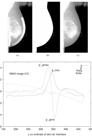
Fig. 5. MIAS image 072 in oblique view with nipple not in profile. (a) The intensities on the original mammogram have been histogram-equalized. (b) Labeled image showing skin-air interface. (c) The estimated nipple position is at the center of the circle. (d) Plot ofg; g0; ; and 0againsty coordinate of skin-air interface. There is a clear maximum and the nipple is estimated aty = 344; the radiologist-determined position is y = 343:
of the maximum or minimum were taken to be integers, or rounded to the nearest integer as well. This would result in some loss of precision and accuracy as rounding errors propagate. There is a possibility, therefore, that results could be in error by at least one pixel in either direction. This is not a serious shortcoming because the method is intended to be simple and its results are constrained in accuracy by the image resolution in any case.
Because the coordinate is used as the independent vari-able, the error will be higher when the slope of the skin-air interface gives rise to large changes in nipple position for small changes in This occurs where the skin-air interface makes a small angle with the positive -direction. The solution to this
would be to use test points that are located at unit increments
along the border rather than along the axis. Again, in the interests of simplicity, this was not done.
Although we have distinguished between the nipple being in profile and the nipple not being in profile, there is actually a gradual transition from one to the other where the nipple may be in profile in varying degrees across different images. On the - curve, this would represent the gradual merging of the two separate peaks as in Fig. 4(d) to the single peak as in Fig. 5(d).
(a) (b) (c)
(d)
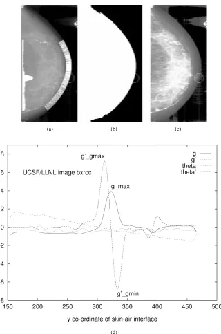
Fig. 6. UCSF/LLNL image bxrcc in cranio-caudal view with nipple not in profile. (a) The intensities on the original mammogram have been transformed logarithmically for display. (b) Labeled image showing skin-air interface. (c) The image has been histogram-equalized for display; note the uneven background. The estimated nipple position is at the center of the circle. (d) Plot ofg; g0; ; and 0againsty coordinate of skin-air interface. There is a clear maximum and the nipple is estimated at y = 323; the radiologist-determined position is y = 324:
result, computed from the positions of the global maximum and minimum of , may not be reliable.
E. Error Analysis
Because of the different image resolutions, the error analysis is done separately for the MIAS and UCSF/LLNL images. For the MIAS images, with image 051 included the mean error is 2.56 pixels or 1.03 mm and the rms error, 7.08 pixels or 2.83 mm. With image 051 excluded, the mean error is 0.93 pixels or 0.37 mm; and the rms error, 2.22 pixels or 0.89 mm. For the UCSF/LLNL images, the mean error is zero pixels and the rms error is 1.66 pixels or 0.70 mm. Thus, in 23 out
of 24 images (96%) across two databases and two views, at resolutions of 400 or 420 m per pixel, the rms error in the -direction between the radiologist-located nipple position and the computer-estimated position was less than 1 mm. This is
an order of magnitude better than the results reported by Yin
et al. [5] on images of similar resolution.
F. Timing of Program
G. Exceptions
In cases where imaging conditions, image quality or ab-normality due to benign or malignant processes modify the intensity profile or lead to an ill-defined skin air interface, this method could fail.
H. Likely Reasons for the Observed Intensity Changes
The observed intensity pattern and its behavior near the nipple invite comment. The discussion in this section is conjectural in that it is not substantiated by a model based on experimental or calculated values of the attenuation co-efficients for different types of breast tissue. Rather, it is a qualitative analysis that seeks to reconcile the observed pattern with what would be expected given the anatomy, geometry and position of the breast during mammography.
The increase in intensity at the nipple could be anticipated from the convergence of the lactiferous ducts (glandular tissue) draining into it. Also, if the nipple were not in profile, it would be lying atop other tissue and adding to the attenuation (and, therefore, intensity) at that point. Anatomically [15, p. 1447] there is no fat immediately beneath the skin of the areola and nipple. If it is recalled that fat is more radiolucent than glandular tissue, this is one more reason for brighter intensities being observed near the nipple.
If the nipple were in profile, the brightening due to the ductal convergence and absence of fat would still be observed close to the nipple, directed toward the breast. However, the geometry and position would dominate the behavior of intensities at the very edge of the nipple. A nipple in profile would represent a very thin layer of tissue projecting from the rest of the breast. The attenuation of X-rays by this thin tissue layer would be comparatively small, leading to a rather faint image at that point. This is in accord with what is observed—nipples in profile are faintly imaged at their outer extremes.
I. Possible Improvements
The method is sensitive to lack of smoothness in the skin-air interface. If this interface were fitted to smooth functions such as splines, and the fitted boundary used, the results would be less dependent on the fidelity of the initial segmentation.
The use of other features, in addition to the mean of the intensity gradients along the normal [see (2)], such as their variance, needs to be investigated. The reliability measure mentioned in Section V could also be used to drive a feedback loop that would confer greater robustness on the algorithm, which at present is open-loop and cannot iteratively improve on a poor first estimate.
Moreover, the simple algorithm we have described cannot accommodate all the variations that naturally occur across mammograms. The threshold , for example, has already been identified as one source of potential weakness.
The patterns of maxima and minima on the smoothed curves of , , , and plotted against are clear enough for a human observer to guess the correct nipple location from them without difficulty in most cases. This means that the smoothed sequences , , , and are discriminating
features. Because we are essentially recognizing maxima and
minima in the two-dimensional neighborhood of smoothed curves, an adaptive, automatic pattern classifier (rather than a set of hierarchical rules) is likely to succeed in this task of learning from examples and generalizing reliably.
VIII. CONCLUSIONS
We have described a simple method for automatically locating the nipple on mammograms. It has been tested out on 24 images from the MIAS and UCSF/LLNL databases—at resolutions of 400 and 420 m per pixel—representing a spectrum of images: oblique-view, cranio-caudal-view, nipple in profile, nipple not in profile, benign, malignant, normal, fatty, glandular, and dense. It located the nipple correctly and with minimal error in 23 images or 96% of the cases. The rms error for these 23 images was less than 1 mm which is an order of magnitude better than a previously reported result in the literature [5] with images of similar resolution. The results justify the hypothesis and its underlying assumptions made at the beginning of this paper. Because of its simplicity, and because it relies both on the tissue characteristics in the nipple region and on geometry, we believe this method has the potential to be a generic means of locating the nipple automatically, especially when coupled with an automatic classifier. It is fast enough to be part of on-line processing of mammograms by computer.
ACKNOWLEDGMENT
The authors would like to thank Dr T. Johnson, M.B., Ch.B., D.M.R.D., F.R.C.R., F.R.A.C.R., D.D.U., of the Perth Radiological Clinic, for locating the nipple on the mam-mograms and establishing the reference data used in this paper. R. Chandrasekhar would also like to acknowledge helpful discussions with H. Sanderson, W. Li, R. Woodcock, and A. Rasiah. The authors would also like to thank the Mammographic Image Analysis Society (MIAS) of the U.K. and the University of California, San Francisco (UCSF), CA, and Lawrence Livermore National Laboratory (LLNL), Livermore, CA, for making available the two databases of digitized mammograms on which this work is based. Finally, they would like to thank the two anonymous reviewers for their constructive suggestions.
REFERENCES
[1] V. F. Andolina, S. Lill´e, and K. M. Willison, Mammographic Imaging: A Practical Guide. Philadelphia: Lippincott, 1992.
[2] M. J. Homer, Mammographic Interpretation: A Practical Approach. New York: McGraw-Hill, 1991.
[3] E. J. Roebuck and R. W. Blamey, Clinical Radiology of the Breast. London, U.K.: Heinemann Medical Books, 1990.
[4] C. Kimme, B. J. O’Loughlin, and J. Sklansky, “Automatic detection of suspicious abnormalities in breast radiographs,” in Data Structures, Computer Graphics and Pattern Recognition, A. Klinger, K. S. Fu, and T. L. Kunii, Eds. New York: Academic, 1977, pp. 427–447. [5] F.-F. Yin, M. L. Giger, K. Doi, C. J. Vyborny, and R. A. Schmidt,
“Computerized detection of masses in digital mammograms: Auto-mated alignment of breast images and its effect on bilateral-subtraction technique,” Med. Phys., vol. 21, pp. 445–452, Mar. 1994.
[7] J. Suckling, J. Parker, D. R. Dance, S. Astley, I. Hutt, C. R. M. Boggis, I. Ricketts, E. Stamatakis, N. Cerneaz, S.-L. Kok, P. Taylor, D. Betal, and J. Savage, “The Mammographic Image Analysis Society digital mammogram database,” in Digital Mammography: Proc. 2nd Int. Workshop on Digital Mammography, York, England, 10–12 July 1994; A. G. Gale, S. M. Astley, D. R. Dance, and A. Y. Cairns, Eds., Excerpta Medica International Congress Series, vol. 1069. Amsterdam, The Netherlands: Elsevier Science, 1994, pp. 375–378.
[8] University of California, San Francisco and Lawrence Livermore Na-tional Laboratory, (UCSF/LLNL), “UCSF/LLNL high-resolution digital mammogram library.” Available from Ms. Christine Skillern, Lawrence Livermore National Laboratory, P.O. Box 808, L-452, Livermore, CA 94551 USA. (e-mail address:[email protected]), 1996. [9] J. L. Semmlow, A. Shadagopappan, L. V. Ackerman, W. Hand, and F.
S. Alcorn, “A fully automated system for screening xeromammograms,” Comput. Biomed. Res., vol. 13, pp. 350–362, 1980.
[10] A. J. Mendez, P. G. Tahoces, M. J. Lado, M. Souto, J. L. Correa, and J. J. Vidal, “Automatic detection of breast border and nipple in digital
mammograms,” Computer Methods and Programs in Biomedicine, vol. 49, pp. 253–262, May 1996.
[11] L. N. Mascio, Private communictaion, Biomedical Image Processing, Engineering Research Division, Lawrence Livermore National Labora-tory, Livermore, CA, 1996.
[12] R. Chandrasekhar, “Systematic Segmentation of Mammograms,” Ph.D. dissertation, Centre for Intelligent Information Processing Systems, Department of Electrical and Electronic Engineering, The University of Western Australia, Nedlands, WA, Australia, Oct. 1996.
[13] R. Chandrasekhar and Y. Attikiouzel, “Gross segmentation of mammo-grams,” in Bridging Disciplines for Biomedicine: Proc. 18th Annu. Int. Conf., IEEE Engineering in Medicine and Biology Society, Oct. 31–Nov. 3, 1996, Amsterdam, The Netherlands, pp. 1–3, CD–ROM Paper 814, IEEE, 1996.
[14] J. Bradley, “xv, version 3.10a.” Published electronically, 1994. Avail-able via anonymous ftp from ftp.cis.upenn.edu, in the directory pub/xv. [15] P. L. Williams, Ed., Gray’s Anatomy, 37th ed.. London, U.K.: