Numerical Solution of Non-linear Fuzzy Differential Equations using Single Term Walsh Series Technique

(1)

Numerical Solution of Non-linear Fuzzy

Differential Equations using Single Term

Walsh Series Technique

A. EmimalKanaga Pushpam

1,*

P. Anandhan

2

Department of Mathematics, Bishop Heber College, Tiruchirappalli 620 017, Tamilnadu, India

Abstract:This paper presents Single Term Walsh Series Technique (STWS) to obtain the numerical solution of non-linear fuzzy differential equations (FDEs). The applicability of this technique is illustrated through two examples. The numerical results are compared with their exact solutions.

Keywords:

Fuzzy differential equations, non-linear, IVP, STWS.

I. INTRODUCTION

The concept of fuzzy differential equations has been growing rapidly. Recently fuzzy differential equations have gained more attention in the literature. The fuzzy derivative was introduced by Chang and Zadeh [8]. Seikkala and Kaleva[15, 16, 22]have studied fuzzy initial value problems (IVPs).Abbasbandy andAllahviranloo [1 – 5]have proposed the numerical methods such as Taylor, Runge Kutta (RK) and predictor corrector methods for finding the solutions of fuzzy differential equations.Recently, Jayakumar et al. [13, 14] have obtained the numerical solution of fuzzy differential equations by RK method of order five and Adams fifth order Predictor-Corrector method. Kanagarajan et al. [17, 18] have extended the numerical solution of RK method and the dependency problem.

Single Term Walsh Series (STWS) technique was introduced by Rao et al. [21]. Balachandran and Murugesan[6, 7] have applied STWS technique to solve first order system of IVPs. Murugesan and Paul Dhayabaran[19]have extended STWS technique for solving second order singular system of IVPs. Sepehrian and Razzaghi [23] have applied STWS technique to solve time-varying singular nonlinear systems. Emimal and Paul Dhayabaran [9, 20] have proposed the generalized STWS Technique to solve invariant and time-varying system of IVPs of any order “n‟ with “p‟

variables. Emimal and Paul Dhayabaran [10] have applied STWS Technique for solving Stiff Non-linear system: High Irradiance Responses (HIRES) of Photo Morphogenesis. Sekar and Senthilkumar [24] have proposed Single term Haar Wavelet Series for fuzzy differential equations.

The authors have developed generalized Single Term Walsh Series (STWS) technique for

solving higher order linear system of time invariant and time varying fuzzy differential equations [11, 12]. In this paper, the authors have proposed the STWS technique to solve non-linear fuzzy differential equations. In Section II, some basic definitions on fuzzy numbers, fuzzy derivatives and fuzzy Cauchy problem have been provided. In Section III, basic properties of Single Term Walsh serieshave been briefly explained. In Section IV, the STWS Technique for solving non-linear system of IVPs has been provided. In Section V, the STWS Technique has been developed to solve the non-linear fuzzy IVPs. In Section VI, numerical examples has been provided to illustrate the applicability of the STWS technique in solving fuzzy IVPs.

II. PRELIMINARIES

Definition 1

Let us denote

R

_F by the class of all fuzzy subsets of R.

i. e. u: R

[0,1])

satisfying the following properties:

0 0

(i) , is normal,

. . with (x ) 1.

F

u R u

i e x R u

(ii)

u

R

_F, u is convex fuzzy set. i . e . u(tx+(1-t)y) min{u(x), u(y)},

t [0,1], x, y R

(iii)

u

R

_F,u is upper semi continuous on R;

(iv) [ ]u0 {x R; u(x) 0} is compact, where

u

denotes the closure of u.

Then

R

_F is called the space of fuzzy numbers.

Definition 2

We define -level set of u as follows:

[u]

{

x

R

/ u(x)

}, 0

1.

(2)

Definition 3

A fuzzy number in parametric form is an ordered pair of the form

u

[u , u ] where 0<

1

satisfying the following conditions:

1.

u

is a bounded left continuous increasing function over [0, 1], 2.

u

is a bounded right continuous decreasing function over [0,1],

3. u u for all (0,1].

If

u

,

then α is called crisp number.

Definition 4

A fuzzy interval u is said to be a triangular fuzzy interval if its membership has the following form

0, , u( )

, 0,

if x a x a

if a x b b a

x

c x

if b x c c b

if x c and its α-cuts are simply

[u] [a (b a), c (c b)], (0,1].

Definition 5

A mapping

F I

:

E

is Hukuhara differentiable at

0

t T R if for some h₀ 0 the Hukuhara difference

0 0 0 0

( ) ~_h ( ), ( ) ~_h ( ),

F t t F t F t F t t

exist in E for all0 t h₀ and if there exists an

' 0

( )

E

F t

such that

'

0 0

(F(t

) ~

( ))

lim

h

( )

0

t

F t

d

F t

t

and

'

0 0

(F(t ) ~ ( ))

lim h ( ) 0,

t

F t t

d F t

t

the fuzzy set is called the Hukuhara derivative of F at t0.

Definition 6

Ify I: Eis called fuzzy process. We denote

[ ( )]y t [y t y t( ), ( )], t I, 0 1

The Seikkala derivative

y t

'

( )

of a fuzzy process y is defined by

' ' '

[ ( )]y t [(y ) ( ), (t y ) ( )], 0t 1,

provided by this equation defines a fuzzy number

'

( )

E. y t

Definition 7

The fuzzy integral

( ) dt, 0 a b 1

b

a

y t

is defined by

( ) ( ) , ( )

b b b

a a a

y t dt y t dt y t dt

provided the Lebesgue integrals on the proper exist.

Fuzzy Initial Value Problem

Consider the fuzzy IVP

0

0 0

'( ) ( , ( ), [ , ]

( )

y t f t y t t t T

y t y

where y is a fuzzy function of t, f (t, y) is a fuzzy operation of the crisp variable t and the fuzzy variable y,

y

'

is the fuzzy derivative of y and y(t0) = y0 is a

fuzzy number. Thus, we have fuzzy Cauchy problem. The fuzzy function y is denoted as

y [ , ]y y .

It means that the α-level set of y(t) for t [ , ]t T₀ is

0 0 0

[ ( )]

y t

[ ( ; ),

y t

( ; )],

[ ( )]

y t

[ ( ; ),

y t

( ; )],

(0,1].

By Zadeh extension principle, we have the membership function

( , ( ))( )

sup{ ( )( ) | ( , )},

f t y t

s

y t

f t

s

R

so ( , ( ))f t y t is a fuzzy number. From this it follows that

[ ( , ( ))]f t y t [ ( , ( ); ),f t y t f t y t( , ( ); )], (0,1]

where

( , ( ); )

min{ ( , ) /

[ ( ; ),

( ; )]

( , ( ); )

max{ ( , ) /

[ ( ; ),

( ; )]

f t y t

f t u

u

y t

f t y t

f t u

u

y t

We define

( , ( ); ) [t, ( ; ), ( ; )],

( , ( ); ) [t, ( ; ), ( ; )].

f t y t F y t y t

f t y t G y t y t

(3)

A function f t( ),integrable in [0,1),may be approximated using Walsh Series as

0

( ) i i( ),

i

f t f t _(3.1)

where _i( )t is the ith Walsh function and fi is the

corresponding coefficient. In practice, only the first ‘m’ terms are considered, where m is an integral power of 2.

Then from (3.1), we get

1

0

( ) ( ) F ( ),

m

T i i i

f t ; f t ; t

where

0, 1, 1

( )T

m F f f K K f

(3.2)

0 1 1

( )

t

( ( ), ( ),

t

K K

_m

( ))

t

T (3.3)

The coefficientsfi are chosen to minimize the mean

integral square error

1

2

0

( ( )f t FT ( ))t dt, _(3.4)

and are given by

1

0

( ) ( ) ,

i i

f f t t dt _(3.5)

It has been proved that

0

( )

t

T

f t dt

;

F E

t

(3.6)

where E is m x m operational matrix for integration in terms of Walsh function. In Single Term Walsh Series, the matrix E in (3.6) becomes E = 1/2.

IV. STWS TECHNIQUE TO SOLVE NON-LINEAR SYSTEM OF IVPs

Consider the non-linear system of IVPs of the form:

0

'( )

( , ( ), ( ))

(0)

y t

f t y t u t

y

(4.1)

where the non-linear function

f

R

n , the state

y( )

t

R

n, and the control

u t

( )

R

q.

The given function is expanded as STWS in the normalized interval

[0, 1)

, which corresponds to

t

[0, 1 /

m

)

by defining

mt

, m being any integer. Normalising (4.1) by defining

mt

, we get

'( )

( , y( ), ( )),

my

f

u

y(0)

y

₀ (4.2)

Let

y'( )

and

y( )

be expanded by STWS series in the kth interval as

y'( )

= V(k) ₀

( )

and

y( )

= Y(k) ₀

( )

(4.3) Integrating equation (4.3) with the operational matrix for integration E = 1/2, we get

Y(k)=

1

2

V

(k)_{+ y(k-1) and y(k) = V}(k)_{+y(k −1).(4.4)}

Therefore,

( )

0

1 y( )

(

1)

( )

2

k

V

y k

(4.5)

To solve (4.2), we first substitute (4.5) in

( , y( ), ( ))

f

u

.

Then we express the resulting equation by STWS as

( ) ( )

0 0

1

, ( 1) ( ), ( ) ( )

2

k k

f V y k u F

(4.6) Using (4.2), (4.3), (4.5), and (4.6), we get

( ) ( )

.

k k

mV

F

(4.7)

By solving (4.7), the components of V(k)can be obtained. Then by substituting V(k) in equation (4.4), discrete approximations of the state variable can be obtained.

V. STWS TECHNIQUE TO SOLVE NON-LINEAR FUZZY IVPs

Consider the non-linear fuzzy differential equations of the following form:

0 0

y'( )

t

f(t, y(t), u(t)),

y t

( )

y

(5.1)

where the non-linear function f Rn, the fuzzy function y(t) Rn, and the fuzzy crisp control

]

[ ( ;

u t

) [ ( ;

u t

)

,

u t

;

]

R

q

.

Here y'is the fuzzy derivative of y, y₀ is fuzzy numbers and y is fuzzy variable.

The given function is expanded as STWS in the normalized interval [0, 1), which corresponds to t [0, 1/m) by defining = mt, m being a crisp number. Normalising the above equation by defining

= mt, we get

'( )

( , y( ), ( )),

my

f

u

y(t )

₀

y

₀ (5.2)

Let

[y'( )] [y'( ), y'( )]

and

[y( )] [y( ), y( )]

be expanded by STWS series

in the kth interval as

( )

1 0

y '( ) _V k ( )_, ( )

0

y( )

y

k

( )

and

( )

2 0

'( ) k ( )

y V y( ) y( )k ₀( ) (5.3)

Integrating equation (5.3) with the operational matrix

for integration E =

1

2

, we get

( )

( ) ( ) ( )

1 2

( ) ( )

1 2

1 1

( 1), ( 1)

2 2

( ) ( 1), ( ) ( 1)

k

k k k

k k

y V y k y V y k

y k V y k y k V y k

(4)

( )

1 0

( )

2 0

1

y( ) ( 1) ( )

2 1

( ) ( 1) ( )

2 k

k

V y k

y V y k

(5.5)

To solve (5.2), we first substitute (5.5) in ( , y( ), ( ))

f u . The resulting equation of STWS is

( ) ( )

1 0 0

1

, ( 1) ( ), ( ) ( )

2

k k

f V y k u F and

( ) ( )

2 0 0

1

, ( 1) ( ), ( ) ( )

2

k k

f V y k u G (5.6)

Using (5.2), (5.3), (5.5), and (5.6), we get

( ) ( ) ( ) ( )

1 , 2

k k k k

mV F mV G (5.7)

By substituting ( ) ( ) 1 and 2

k k

V V in equation (5.4),

discrete approximations of the state variable can be obtained.

VI. NUMERICAL EXAMPLES

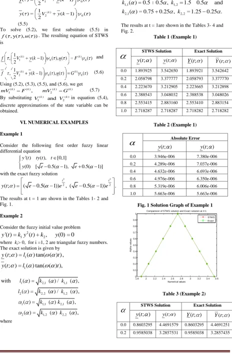
Example 1

Consider the following first order fuzzy linear differential equation

'( ) ( ), [0,1]

(0) [ 0.5( 1), 0.5( 1)]

y t ty t t

y e e

with the exact fuzzy solution

2 2

( ; )

(

0.5(

1))

, (

0.5(

1))

.

t t

y t

e

The results at t = 1 are shown in the Tables 1- 2 and Fig. 1.

Example 2

Consider the fuzzy initial value problem

2

1 2

'( )

( )

,

(0)

0 y t

k y t

k

y

where ki> 0, for i =1, 2 are triangular fuzzy numbers.

The exact solution is given by

1

( ; )

( ) tan( ( ) ) ,

( ; )

( ) tan( ( ) ),

y t

l

t

y t

l

t

1 2,1 1,1

2 2,2 1,2

1 1,1 2,1

2 1,2 2,2

with

( )

( ) /

( ),

( )

( ) /

( ),

( )

( ),

( )

( ),

l

k

l

k

where

1,1 1,2

2,1 2,2

( )

0.5 0.5 ,

1.5

0.5 and

( )

0.75 0.25 ,

1.25 0.25 .

k

The results at t = 1are shown in the Tables 3- 4 and Fig. 2.

Table 1 (Example 1)

STWS Solution Exact Solution

( ; )

y t

y t( ; )

Y t

( ; )

Y t( ; )

0.0 1.893925 3.542650 1.893921 3.542642

0.2 2.058798 3.377777 2.058793 3.377770

0.4 2.223670 3.212905 2.223665 3.212898

0.6 2.388543 3.048032 2.388538 3.048026

0.8 2.553415 2.883160 2.553410 2.883154

1.0 2.718287 2.718287 2.718282 2.718282

Absolute Error

( ; )

y t

( ; )

0.0 3.946e-006 7.380e-006

0.2 4.289e-006 7.037e-006

0.4 4.632e-006 6.693e-006

0.6 4.976e-006 6.350e-006

0.8 5.319e-006 6.006e-006

1.0 5.663e-006 5.663e-006

Fig. 1 Solution Graph of Example 1

STWS Solution Exact Solution

( ; )

y t

y t( ; )

Y t

( ; )

Y t( ; )

0.0 0.8603295 4.4691579 0.8603295 4.4691251

0.2 0.9585038 3.2857531 0.9585038 3.2857435 1.8 2 2.2 2.4 2.6 2.8 3 3.2 3.4 3.6 0

0.1 0.2 0.3 0.4 0.5 0.6 0.7 0.8 0.9 1

Numerical values

A

lp

h

a

v

a

lu

e

s

Comparision of STWS solution and Exact solution at t=1

(5)

0.4 1.0714393 2.5919473 1.0714393 2.5919439

0.6 1.2038061 2.1331447 1.2038061 2.1331433

0.8 1.3623815 1.8051551 1.3623814 1.8051545

1.0 1.557408 1.557408 1.557408 1.557408

Absolute Error

( ; )

y t

( ; )

0.0 1.956e-008 3.280e-005

0.2 2.192e-008 9.626e-006

0.4 1.791e-008 3.400e-006

0.6 1.568e-009 1.312e-006

0.8 5.643e-008 5.164e-007

1.0 1.919e-007 1.919e-007

Fig. 2 Solution Graph of Example 2

VII. CONCLUSION

In this paper, STWS method has been proposed to solve the non- linear fuzzy IVPs. The effectiveness of this method has been illustrated through two examples. From the tables, it is observed that the absolute error is very small. The recursive algorithm is easy to implement and suitable in finding solution for any length of time. This suggests that STWS technique is suitable for solving non-linear fuzzy IVPs.

REFERENCES

[1] S. Abbasbandy, T. Allahviranloo, Numerical solution of fuzzy differential equation by Taylor method, Journal of Computational Methods in Applied mathematics, 2 (2002) 113-124.

[2] S. Abbasbandy, T. Allahviranloo, Numerical solution of fuzzy differential equation, Mathematical and Computational Applications, 7 (2002) 41-52.

[3] S. Abbasbandy, T. Allahviranloo, Numerical solution of fuzzy differential equation by Runge-Kutta method,

Nonlinear Studies, 11 (2004) 117-129.

[4] T. Allahviranloo, N. Ahmady, E. Ahmady, Numerical solution of fuzzy differential equations by predictor-Corrector method, Information Sciences, 177 (2007) 1633-1647.

[5] T. Allahviranloo, S. Abbasbandy N. Ahmady, E. Ahmady, Improved predictor-Corrector method for solving fuzzy initial value problems, Information Sciences, 179 (2009) 945-955.

[6] K. Balachandran, K. Murugesan, Analysis of different systems via Single term Walsh series method, International Journal of Computer Mathematics, 33 (1990) 171–179. [7] K. Balachandran, K. Murugesan, Analysis of non-linear

singular systems via STWS method, International Journal of Computer Mathematics, 36, (1990) 9–12.

[8] S. L. Chang and L. A. Zadeh, On Fuzzy Mapping and Control, IEEE Trans. Systems, Man, and Cybernet, 2 (1972) 30-34.

[9] A. EmimalKanagaPushpam , D. Paul Dhayabaran, E.C. Henry Amirtharaj, Numerical solution of higher order systems of IVPs using generalized STWS technique, Applied Mathematics and Computation, 180 (2006)200–205. [10] A. EmimalKanagaPushpam, D. Paul Dhayabaran, An

Application of STWS Technique in Solving Stiff Non-linear System: High Irradiance Responses (HIRES) of Photo morphogenesis, Recent Research in Science and Technology,

3(6) (2011) 47-53.

[11] A. EmimalKanagaPushpam, P. Anandhan, Numerical Solution of Higher Order Linear Fuzzy Differential Equations using Generalized STWS Technique,

International J. Innovative Research in Science, Eng. and Technology (IJIRSET), 5(3) (2016) 3862 - 3869.

[12] A. EmimalKanagaPushpam, P. Anandhan, Solving Higher Order Linear System of Time Varying Fuzzy Differential Equations using Generalized STWS Technique,

International Journal of Science and Research, 5(4) (2016) 57 – 61.

[13] T. Jayakumar, D. Maheshkumar, K. Kanagarajan, Numerical solution of fuzzy differential equations by Runge-Kutta method order five, International Journal of Applied Mathematical Science, 6 (2012) 2989-3002.

[14] T. Jayakumar, C.Raja, T.Muthukumar, Numerical solution of fuzzy differential equations by Adams fifth order predictor-corrector method, International Journal of Mathematics Trends and Technology (2014) 1-18.

[15] O. Kaleva, Fuzzy Differential Equations, Fuzzy Sets Systems, 24 (1987) 301-317.

[16] O. Kaleva, The Cauchy problem for Fuzzy Differential Equations, Fuzzy Sets Systems, 35 (1990) 389-396. [17] K. Kanagarajan, S. Muthukumar, S. Indrakumar Numerical

solution of fuzzy differential equations by Extended Runge-Kutta Method and the Dependency Problem, International Journal of mathematics Trends and Technology 6(2014) 113-122.

[18] K. Kanagarajan, M. Sambath, Numerical solution of fuzzy differential equations by third order Runge-Kutta method,

International Journal of Applied Mathematics and Computation, 2 (2010) 1-10.

[19] K. Murugesan, D. P. Dhayabaran, D. J. Evans, Analysis of second order multivariable linear system using Single-term Walsh series technique and Runge Kutta method,

International Journal of Computer Mathematics, 72 (1999) 367–374.

[20] D. Paul Dhayabaran, A. EmimalKanagaPushpam, E.C. Henry Amirtharaj, Generalized STWS technique for higher order time-varying singular systems, International Journal of Computer Mathematics, 84 (2007) 395–402.

[21] G. P. Rao, K. R. Palanisamy, T. Srinivasan, Extension of computation beyond the limit of normal interval in Walsh series analysis of dynamical systems, IEEE. Trans. Automat. Contr., 25(1980) 317–319.

[22] S. Seikkala, On the Fuzzy Initial Value Problem, Fuzzy Sets Systems, 24 (1987)319-330.[

[23] B. Sepehrian and M. Razzaghi, Solution of time-varying singular nonlinear systems by Single-term Walsh series,

Mathematical Problems in Engineering 2003, 3 (2003), 129–136.

[24] S. Sekar, S. Senthilkumar, Single Term Haar Wavelet series forfuzzy differential equations, International Journal of Mathematics Trends and Technology 4 (9)( 2013), 181-188. 0.5 1 1.5 2 2.5 3 3.5 4 4.5

0 0.1 0.2 0.3 0.4 0.5 0.6 0.7 0.8 0.9 1

Numerical Values

A

lp

h

a

V

a

lu

e

s

Comparision of STWS Solution and Exact Solution at t=1