The Thirty-Third AAAI Conference on Artificial Intelligence (AAAI-19)
HyperAdam: A Learnable Task-Adaptive Adam for Network Training
Shipeng Wang, Jian Sun,
∗Zongben Xu
School of Mathematics and Statistics, Xi’an Jiaotong University, Xi’an, 710049, China [email protected],{jiansun, zbxu}@xjtu.edu.cn
Abstract
Deep neural networks are traditionally trained using human-designed stochastic optimization algorithms, such as SGD and Adam. Recently, the approach of learning to optimize network parameters has emerged as a promising research topic. However, these learned black-box optimizers some-times do not fully utilize the experience in human-designed optimizers, therefore have limitation in generalization ability. In this paper, a new optimizer, dubbed asHyperAdam, is pro-posed that combines the idea of “learning to optimize” and traditional Adam optimizer. Given a network for training, its parameter update in each iteration generated by HyperAdam is an adaptive combination of multiple updates generated by Adam with varying decay rates . The combination weights and decay rates in HyperAdam are adaptively learned de-pending on the task. HyperAdam is modeled as a recurrent neural network with AdamCell, WeightCell and StateCell. It is justified to be state-of-the-art for various network training, such as multilayer perceptron, CNN and LSTM.
1
Introduction
Deep learning approach has exhibited strong capabilities in data representation (LeCun, Bengio, and Hinton 2015), non-linear mapping (Sutskever, Vinyals, and Le 2014), distribu-tion learning (Goodfellow et al. 2014), etc. Deep learning not only has wide applications in a broad field of academi-cal studies, such as image analysis (He et al. 2016), speech recognition (McMahan and Rao 2018), robotics (Lillicrap et al. 2016), inverse problem (Yang et al. 2016), but also draws attention of industry for realization in products.
One challenge in deep learning is the effective optimiza-tion of deep network parameters, required to be generaliz-able to varying network architectures, e.g., network type, depth, width, non-linear activation functions. For a neural networkf(x;w), the aim of network training is to find the optimal network parametersw∗ ∈ Rp to minimize
empir-ical loss between the network output given inputxi ∈ Rd
and the corresponding target labelyi∈Rb:
w∗ = arg min
w Σ N
i=1l(f(xi;w), yi), (1)
∗
corresponding author
Copyright c2019, Association for the Advancement of Artificial Intelligence (www.aaai.org). All rights reserved.
where{(xi, yi)}Ni=1is the training set. For a deep neural
net-work, the dimension pand number of training dataN are commonly large in real applications.
The network, as a learning machine, is referred to as a
learner, the loss for network training is defined as an op-timizee, and the optimization algorithm to minimize opti-mizee is referred to as anoptimizer. For example, a gradient-based optimizer can be written as a functionOthat maps the gradientgtto network parameter updatedtint-th iteration:
dt(Θ) =O(gt,Ht;Θ), (2)
whereHtrepresents the historical gradient information and Θrepresents the hyperparameters of the optimizer.
The human-designed optimizers, such as stochastic gra-dient descent (SGD) (Robbins and Monro 1951), RMSProp (Tieleman and Hinton 2012), AdaGrad (Duchi, Hazan, and Singer 2011), AdaDelta (Zeiler 2012) and Adam (Kingma and Ba 2015), are popular in network training. They have well generalization ability to various network architectures and tasks. Adam takes the statistics of gradients as the histor-ical information recursively accumulated with constant de-cay rates (i.e.,β, γin Alg. 1). Though universal, Adam suf-fers from unsatisfactory convergence in some cases because of the constant decay rates (Reddi, Kale, and Kumar 2018).
Recently, “learning to optimize”, i.e., learning the opti-mizer by data-driven approach, triggered the interest of com-munity. The optimizer (Andrychowicz et al. 2016) outputs the update vector by RNN, whose generalization ability is improved by two training tricks (Lv, Jiang, and Li 2017). This idea is also applied to optimizing derivative-free black-box functions (Chen et al. 2017). From the perspective of reinforcement learning, the optimizer is taken as policy (Li and Malik 2016). Though faster in decreasing training loss than the traditional optimizers in some cases, the learned op-timizers do not always generalize well to diverse variants of learners. Moreover, they can not be guaranteed to output a descent direction in each iteration for network training.
Algorithm 1Adam Optimizer
Require:
1: Initialized parameterw0, step sizeα, batch sizeNB. 2: Exponential decay ratesβ, γ; dataset{(xi, yi)}Ni=1. Initialize: m0= 0, v0= 0.
3: for allt= 1, . . . , T do
4: Draw random batch{(xik, yik)}
NB
k=1from dataset 5: gt= ΣNk=1B∇l(xik, yik, wt−1)
6: mt=βmt−1+ (1−β)gt .moving average
7: vt=γvt−1+ (1−γ)g2t
8: m˜t= 1m−βtt,˜vt= 1−vtγt .correcting bias
9: mˆt= √m˜v˜t
t+ε
10: wt=wt−1−αmˆt
11: end for
12: returnfinal parameterwT.
idea, AdamCell and WeightCell are respectively designed to generate candidate updates and weights to combine them, conditioned on the output of StateCell for modeling task-dependent state. As a recurrent neural network, parameters of HyperAdam are learned by training on a meta-train set.
The main contribution of this paper is two-fold. First, to the best of our knowledge, this is a first task-adaptive opti-mizer taking merits of adaptive moment estimation approach (i.e., Adam) and learning-based approach in a single frame-work. It opens a new door to design learning-based opti-mizer inspired by traditional human-designed optiopti-mizers. Second, extensive experiments justify that the learned Hy-perAdam outperforms traditional optimizers, such as Adam and learning-based optimizers for training a wide range of neural networks, e.g., deep MLP, CNN, LSTM.
2
Related Works
2.1
Learning to Optimize
With the goal of facilitating learning of novel tasks, meta-learningis developed to extract knowledge from observed tasks (Amit and Meir 2018; Ren et al. 2018; Finn et al. 2017; Snell, Swersky, and Zemel 2017; Wichrowska et al. 2017; Santoro et al. 2016; Daniel, Taylor, and Nowozin 2016).
This paper focuses on the meta-learning task of optimiz-ing network parameters, commonly termed as “learnoptimiz-ing to optimize”. It originates from several decades ago (Schmid-huber 1992; Naik and Mammone 1992) and is developed af-terwards (Hochreiter, Younger, and Conwell 2001; Younger, Hochreiter, and Conwell 2001). Recently, a more general op-timizer that conducts parameter update by LSTM with gradi-ent as input is proposed in (Andrychowicz et al. 2016). Two effective training techniques, “Random Scaling” and “Com-bination with Convex Functions”, are proposed to improve the generalization ability (Lv, Jiang, and Li 2017). Subse-quently, several works use RNN to replace certain process in some optimization algorithms, e.g., variational EM (Marino, Yue, and Mandt 2018), ADMM (Liu et al. 2018). In (Chen et al. 2017), RNN is also used to optimize derivate-free black-box functions.
Algorithm 2Task-Adaptive HyperAdam
Require:
1: Initialized parameterw0, step sizeα, batch sizeNB.
2: Dataset{(xi, yi)}Ni=1. Initialize:
3: m0,v0,βˆ0,γˆ0,s0=0∈Rp×J,1∈Rp×J,ε=1e-24 . 4: for allt= 1, . . . , T do
5: Draw random batch{(xik, yik)}
NB
k=1from dataset 6: gt= ΣNk=1B∇l(xik, yik, wt−1)
7: Gt= [gt, . . . , gt] .Gt∈Rp×J 8: st=Fh(st−1, gt;Θh) .current state
9: βt,[βt1, . . . , βtJ] =Fu(st,mt−1;Θu)
10: γt,[γt1, . . . , γtJ] =Fr(st,mt−1;Θr)
11: mt=βtmt−1+ (1−βt)Gt
12: vt=γtvt−1+ (1−γt)G2t
13: βˆt=βtβˆt−1+ (1−βt)1
14: γˆt=γtγˆt−1+ (1−γt)1
15: m˜t=mt/βˆt,v˜t=vt/γˆt, .correcting bias
16: mˆt,[ ˆm1t, . . . ,mˆJt] =
˜
mt
√ ˜
vt+ε .moment field
17: ρt,[ρ1t, . . . , ρJt] =Fq(st;Θq) .weight field
18: dt= ΣJj=1ρ
j tmˆ
j t
19: wt=wt−1−αdt
20: end for
21: returnfinal parameterwT.
These pioneering learning-based optimizers have shown promising performance, but did not fully utilize the expe-rience in human-designed optimizers, and sometimes have limitation in generalizing to variants of networks. The pro-posed optimizer, HyperAdam, is a learnable optimizer but with architecture designed by generalizing traditional Adam optimizer. In the evaluation section, the HyperAdam is jus-tified to have better generalization ability than previous learning-based optimizers for training various networks.
2.2
Adam Method
Vanilla SGD has been improved by adaptive learning rates for each parameter (e.g., AdaGrad, AdaDelta, RMSProp) or (and) Momentum (Tseng 1998). Adam (Kingma and Ba 2015) is an adaptive moment estimation method combining these two techniques, as illustrated in Alg. 1. Adam takes unbiased estimation of second moment of gradients as the ingredient of the coordinate-wise learning rates, and the un-biased estimation of first moment of gradients as the basis for parameter updating. The bias is caused by the initializa-tion of mean and uncentered variance during online moving average with decay rates (i.e., β, γin Alg. 1). It is easy to verify that the parameters update generated by Adam is in-variant to the scale of gradients when ignoringε.
Optimizee wt−2 + wt−1 + wt + wt+1
Lt−2 Lt−1 Lt
Optimizer H O t−2
O
Ht−1
O
Ht Ht+1
dt−1 dt dt+1 gt−1 gt gt+1
gt
StateCell
s1 t . . . sJt
ˆ
m1
t . . . mˆJt ρ1t . . . ρJt
AdamCell WeightCell
dt
Combination
s1
t−1 . . . sJt−1 m1
t−1. . .mJt−1
s1 t s
J t . . . m1
t . . . mHt
Ht−1 Ht
Moment field Weight field
Figure 1: Computational graph of HyperAdam.Orepresents the optimizer.gtis the gradient of the optimizeeLanddtis the update vectors. The historical informationHtconsists of the first moment and previous task state.
(Wolpert 1992) of HyperAdam that combines multiple can-didate updates can potentially find more reliable descent di-rections. These techniques are justified to be effective for improving the baseline Adam in evaluation section.
3
HyperAdam
In this section, we introduce the general idea, algorithm and network architecture of the proposed HyperAdam.
3.1
General Idea
Adam is non-adaptive because its hyperparameters (decay ratesβandγin Alg. 1) are constant and set by hand when optimizing a network. According to Alg.1, different hyper-parameters make the parameter updates different both in di-rection and magnitude. Our proposed HyperAdam improves Adam as follows. First, Adam in HyperAdam is designed with multiple learned task-adaptive decay rates and to gen-erate multiple candidate parameter updates with correspond-ing decay rates in parallel. Second, HyperAdam combines these parameter updates to get the final parameter update using adaptively learned combination weights.
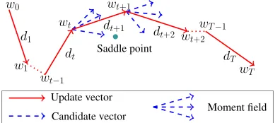
As illustrated in Fig. 2, at a certain point, e.g., wt in parametric space, multiple update vectors are generated by Adam with different decay rates. The final updatedt is an adaptive combination of these candidate vectors. Consider-ing that, for a deep neural network (Dauphin et al. 2014), there exist abundant saddle points surrounded by high loss
w0
d1
w1
wt−1
wt
dt Saddle point
wt+1
dt+1 d
t+2 wt+2
dT
wT−1
wT
Update vector
Candidate vector Moment field
Figure 2: An illustration of parameter optimization of a learner using proposed HyperAdam algorithm.
plateaus, a certain candidate update vector may point to a saddle point, but an adaptive combination of several candi-date vectors may potentially relieve the possibility of getting stuck in saddle point.
3.2
Task-Adaptive HyperAdam
Based on the above idea, we design a task-adaptive Hyper-Adam in Alg. 2. In iteration t, first, the current state st is determined bystate functionFhwith current gradientgtand previous statest−1as inputs in line 8. Then in lines 9-16,J
candidate update vectors mˆjt are generated by Adam with J pairs of decay rates (βtj, γtj) which are adaptive to the current statestviadecay-rate functionsFuandFr. Mean-while, J task-adaptive weight vectors ρjt are generated by
weight functionFq with the current statestas input in line 17. Finally, the final update vector dt is a combination of the candidate updates weighted by weight vectors in line 18.
ˆ
mtcontaining candidate updates and ρtcontaining weight vectors are calledmoment fieldandweight fieldrespectively. As illustrated in the left of Fig. 1, HyperAdam, as an op-timizer, is a recurrent mappingOiteratively generating pa-rameter updates. The right of Fig. 1 shows the graphical dia-gram of HyperAdam having four components. The StateCell corresponds to thestate functionFhoutputting the current statest = [s1t, . . . , sJt]. With the current state as basis, the
moment field and weight field are produced by AdamCell and WeightCell respectively. The final updatedt is gener-ated in the “Combination” block. We next introduce these components.
gt
Normalization Preprocessing LSTM
st−1
st
StateCell
StateCell The current state st = [s1t, . . . , sJt] is deter-mined by the gradientgtand previous task statest−1in the
StateCell implementing the state function Fh in line 8 of Alg. 2. The diagram of StateCell is illustrated in Fig. 3. After normalized with its Euclidean norm, the gradient is prepro-cessed by a fully connected layer with Exponential Linear Unit (ELU) (Clevert and and 2016) as activation function. Following preprocessing, the gradient together with the pre-vious task statest−1are fed into LSTM (Reiter and
Schmid-huber 1997) to generate the current statest.
AdamCell AdamCell is designed to implement lines 9-16 in Alg. 2 for generating moment field, i.e. a group of update vectors. We first analyze these lines. Task-adaptive decay rates βt,γt are generated by decay-rate functionsin lines 9-10, with which the biased estimations of first and second moment of gradientsmt,vtare recursively accumulated in lines 11-12. The bias factors βˆt,γˆt are computed in lines 13-14. Finally, moment field is produced with unbiased esti-mations of first and second moment of gradients in line 16.
Note that the accumulatedβˆt(line 13 of Alg. 2) is equiv-alent to 1−βt when βis constant based on lemma 1. It also holds forγˆt. Therefore, we can derive that each com-ponent in moment field (line 16 of Alg. 2) is equivalent to a parameter update produced by Adam in line 9 of Alg. 1.
Lemma1 βˆt=ββˆt−1+ (1−β)withβˆ0 = 0is the online
formula ofβˆt= 1−βt.
Proof1 See proof in supplementary material.
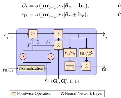
If we denoteCt = [mt,vt,βˆt,γˆt],Ft = [βt,γt,βt,γt] andC˜t = [Gt,G2t,1,1](1 ∈ Rp×J), based on lemma 1, lines 11-14 in Alg. 2 can be expressed in the following com-pact formula resembling cell state updating in LSTM:
Ct=FtCt−1+ (1−Ft)C˜t. (3)
Thus we construct AdamCell, a structure like LSTM, to con-duct lines 9-16 in Alg. 2 as illustrated in Fig. 4.Ft deter-mines how much historical information would be forgot like the forget gate in LSTM. We define thedecay-rate functions
Fr, Fuin Alg. 2 to be in parametric forms:
βt=σ([m0t−1,st]θu+bu), (4)
γt=σ([m0t−1,st]θr+br), (5)
Ct−1 Ct
mt−1
Pointwise Operation Neural Network Layer
+
Normalization
st
σ σ
Ft
1−Ft
(Gt,G2t,1,1)
vt/γˆt mt/βˆt
1 √
·+ mˆ
t
Figure 4: Diagram of AdamCell. The neural network layer corresponds to the decay-rate functionsFu, Frin Alg. 2.
withθu,θr ∈R2J×J,bu = [bu, . . . , bu]T ∈ Rp×J,br =
[br, . . . , br]T ∈ Rp×J andm0t−1 = [
m1t km1
tk2, . . . ,
mJt kmJ
tk2] ∈ Rp×J, whereΘu = {θu, bu}, Θr ={θr, br}are learnable parameters. The decay-rate functions Fr,Fu output decay ratesβt = [β1t, . . . βtJ]andγt = [γt1, . . . γtJ] respectively, and each pair of decay rates(βtj, γtj)determines a candidate update vectormˆjtgenerated by Adam.
WeightCell WeightCell is designed to implement the
weight function Fq (line 17 in Alg. 2) which outputs the
weight field with the current statest as input. The weight function is a one-hidden-layer fully connected network with ELU as activation function:
ρt=ELU(stθq+bq), (6)
withθq ∈ RJ×J andbq = [bq, . . . , bq]T ∈ Rp×J where
Θq={θq, bq}are learnable parameters.
We choose ELU instead of ReLU as activation function to ensure that the weights are not always positive, since some candidate vectors in themoment fieldmay not be favorable because of pointing to a bad direction.
Combination The final update dt is the combination of the candidate update vectors in moment field with weight vectors in weight field (line 18 in Alg. 2):
dt= ΣJj=1ρ
j tmˆ
j
t. (7)
Parameter sharing It can be verified that the different co-ordinates of parameter w and intermediate terms such as
st,βt,γtshare the hyperparameterΘ ={Θh, Θq, Θr, Θu} of HyperAdam. For example, different rows of βt in Eqn. (4), corresponding to different coordinates ofw, share hyperparametersΘu. Moreover,J candidate update vectors are generated in parallel by matrix operations. Consequently, HyperAdam can be applied to training networks with vary-ing dimensional parameters in parallel.
Scale invariance To achieve the scale invariance property same as traditional Adam, the gradient gt and mjt (j =
1, . . . , J) are normalized by their Euclidean norms in State-Cell and AdamState-Cell (see proof in supplementary material).
4
Learning HyperAdam
We train HyperAdam on a meta-train set consisting of learner (i.e., network in this paper) coupled with correspond-ing optimizee (loss for traincorrespond-ing learner) and dataset, which is implemented by TensorFlow. We aim to optimize the param-eters of HyperAdam to maximize its capability in training learners over the meta-train set. We expect that the learned HyperAdam can be generalized to optimize more complex networks beyond the learners in meta-train set. We next in-troduce the training process in details.
Meta-train set consists of triplets of learnerf, optimizee L, and dataset D = {X, Y}, where X = {xi}Ni=1 and
Y = {yi}Ni=1 represent the data set and corresponding
la-bel set. The HyperAdam parameter set Θ is optimized by minimizing the expected cumulative regret (Andrychowicz et al. 2016) on the meta-train set:
L(Θ) =EL[
1 TΣ
T
wherewt(Θ) =wt−1(Θ)−αdt(gt, Θ)is network parame-ter of learnerfat iterationtwhen optimized by HyperAdam with parametersΘ ={Θh, Θq, Θr, Θu}.f(X;wt(Θ)) de-notes the network output of learner f on dataset Dwhen network parameter iswt(Θ), andL(·,·)is an optimizee, i.e., the loss for training learnerf. Therefore,L(Θ)defines the expectation of the cumulative loss over meta-train set. Mini-mizingL(Θ)is to find optimal parameter for HyperAdam to reduce training lossL(i.e., optimizee) as lower as possible. As in (Lv, Jiang, and Li 2017), the learner f is simply taken as a forward neural network with one hidden layer of 20 units and sigmoid as activation function. The optimizeeL is defined asL(f(X;w), Y) = ΣN
i=1l(f(xi;w), yi)wherel is the cross entropy loss for the learnerfwith a minibatch of 128 random images sampled from the MNIST dataset (Le-Cun et al. 1998). We set the learning rateα = 0.005and maximal iterationT = 100indicating the number of opti-mization steps using HyperAdam as an optimizer. The num-ber of candidate updatesJ is set to be 20.
HyperAdam can be seen as a recurrent neural network iteratively updating network parameters. Therefore we can optimize parameterΘ of HyperAdam using BackPropaga-tion Through Time (Werbos 1990) by minimizing L(Θ)
with Adam, and the expectation with respect toLis approx-imated by the average training loss for learnerfwith differ-ent initializations. TheT = 100steps are split into 5 periods of 20 steps to avoid gradient vanishing. In each period, the initial parameterw0and initial hidden stateHare initialized
from the last period or generated if it is the first period. Two training tricks proposed in (Lv, Jiang, and Li 2017) are used here. First, in order to make the training easier, a k-dimensional convex functionh(z) = k1kz−ηk2is
com-bined with the original optimizee (i.e., training loss), and this trick is called “Combination with Convex Function” (CC).η and initial value ofzare generated randomly. Sec-ond, “Random Scaling” (RS), helping to avoid over-fitting, randomly samples vectorsc1andc2of the same dimension
as parameter w andz respectively, and then multiply the parameters withc1 andc2 coordinate-wisely, thus the
op-timizee in the meta-train set becomes:
Lext(w, z) =L(f(X;c1w), Y) +h(c2z), (9)
with initial parametersdiag(c1)−1w, diag(c2)−1z.
5
Evaluation
We have trained HyperAdam based on 1-layer MLP (basic MLP), we now evaluate the learned HyperAdam for more complex networks such as basic MLP with different activa-tion funcactiva-tions, deeper MLP, CNN and LSTM.
• Activation functions: The activation function of basic MLP is extended from sigmoid to ReLU, ELU and tanh. • Deep MLP:The number of hidden layers of MLP is
ex-tended to range of[2,10], and each layer has 20 hidden units and uses sigmoid as activation function.
• CNN: Convolution neural networks are with structures ofc-c-p-f(CNN-1) andc-c-p-c-c-p-f-f (CNN-2), where c,pandf represent convolution, max-pooling and fully-connected layer respectively. Convolution kernel is with
size of 3×3and the max-pooling layer is with size of
2×2 and stride 2. CNN-1 and CNN-2 are also trained with batch normalization and dropout respectively. • LSTM: LSTM with hidden state in size of 20 is
ap-plied to sequence prediction task using mean squared er-ror loss as in (Lv, Jiang, and Li 2017). Given a sequence f(0), . . . , f(9)with additive noise, the LSTM is supposed to predict the value off(10). Heref(x) =Asin(wx+φ). The dataset is generated with uniformly random sampling A ∼ U(0,10), w ∼ U(0, π/2), φ ∼ U(0,2π), and the noise is drawn from Gaussian distributionN(0,0.1).
We also evaluate whether our learned HyperAdam can well generalize to different datasets, e.g. CIFAR-10 (Krizhevsky 2009). Moreover, the HyperAdam is trained assuming it it-eratively optimizes network parameters in fixed iterations T = 100, we also evaluate the learned HyperAdam for longer iterative optimization steps as in (Lv, Jiang, and Li 2017). The generalization ability of the networks trained by HyperAdam will be also evaluated preliminarily.
In evaluations, we will compare our HyperAdam with traditional network optimizers such as SGD, AdaDelta, Adam, AdaGrad, Momentum, RMSProp, and state-of-the-art learning-based optimizers including RNNprop (Lv, Jiang, and Li 2017), DMoptimizer (Andrychowicz et al. 2016). For the traditional optimizers, we hand-tuned the learning rates and set other hyperparameters as defaults in TensorFlow. All the initial parameters of learners used in the experiments are sampled independently from the Gaussian distribution. We report the quantitative value as the average measure for training the learner 100 times with random pa-rameter initialization.
5.1
Generalization with Fixed Optimization Steps
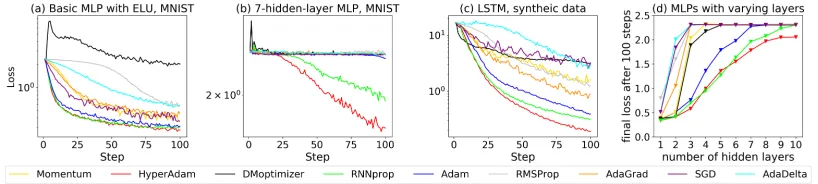
We first assume that the learned HyperAdam optimizes the parameters of learners for fixed optimization stepsT = 100, same as the learning procedure for HyperAdam.Activation functions As shown in Table 1, HyperAdam is tested for training basic MLP with different activation func-tions on MNIST dataset, the loss values in Table 1 show that HyperAdam can best generalize to optimize basic MLP with ReLU, ELU and tanh as activation functions, compared with DMoptimizer and RNNprop. Our HyperAdam also outper-forms the basic Adam algorithm. The DMoptimizer can not well generalize to basic MLP with ELU activation function, which can be also visually observed in Fig. 5(a).
Deep MLP We further evaluate performance of Hyper-Adam on learning parameters of MLPs with varying layer
Activation Adam DMoptimizer RNNprop HyperAdam sigmoid 0.35 0.38 0.34 0.33
ReLU 0.32 1.42 0.31 0.29
ELU 0.31 2.02 0.31 0.28
tanh 0.34 0.83 0.33 0.36
Figure 5: HyperAdam performs best compared with other optimizers on neural networks with different structures.
Figure 6: Comparison of different optimizers for optimizing different CNNs in different optimization steps.
numbers. According to Fig. 5(d), for different number of hidden layers ranging from 1 to 10, HyperAdam always performs significantly better than Adam and DMoptimizer. Compared with RNNprop, HyperAdam is better in general, especially for deeper MLP with more than 6 layers. The loss curves in Fig. 5(b) of different optimizers for MLP with 7 hidden layers illustrate HyperAdam is significantly better.
LSTM As shown in Table 2, the “Baseline” task is to uti-lize one-layer LSTM to predictf(10)on dataset with noise drawn fromN(0,0.1), which is further varied by training on dataset with small noise drawn fromN(0,0.01)(“Small noise”) or using two-layer LSTM (“2-layer”) for prediction. By comparing the loss values in Table 2, our HyperAdam can better decrease the training losses than the compared op-timizers, i.e., Adam, DMoptimizer, RNNprop, HyperAdam. Specifically, Fig. 5(c) shows an example for the comparison in task of “Small noise”.
Figure 7: HyperAdam with 10000 optimization steps. Train-ing curves by DMoptimizer, AdaGrad, RMSProp, AdaDelta, Momentum and SGD coincide in the left figure.
Task Adam DMoptimizer RNNprop HyperAdam Baseline 0.65 3.10 0.49 0.42
Small noise 0.39 3.06 0.32 0.19
2-layer 0.51 2.05 0.27 0.26
Table 2: Performance on different sequence prediction tasks.
CNN Figure 6(a)-(b) compare training curves of CNN-1 and CNN-2 on MNIST using different optimizers. Figure 6(e)-(f) compare training curves of CNN-1 with batch nor-malization and CNN-2 with dropout on CIFAR-10 respec-tively. In these figures, DMoptimizer and RNNprop do not always perform well or even fail while HyperAdam can ef-fectively decrease the training losses in different tasks.
5.2
Generalization to Longer Horizons
We have evaluated HyperAdam for optimizing different learners in fixed optimization steps (T = 100), same as the meta-training phase. We now evaluate HyperAdam for its effectiveness in running optimization for longer steps.
Deep MLP Figure 7(a) illustrates the training curves of MLP with 9 hidden layers on MNIST using different op-timizers for 10000 steps. DMoptimizer and almost all tra-ditional optimizers, including SGD, Momentum, AdaGrad, AdaDelta and RMSProp, fail to decrease the loss. Our Hy-perAdam can effectively decrease the training loss.
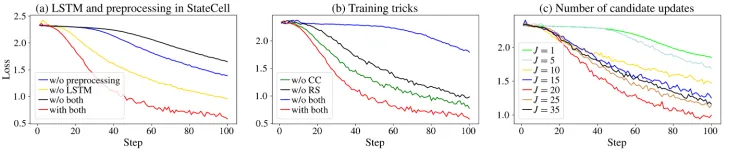
Figure 8: Ablation study for the number of candidate updates, training tricks and structure in StateCell. CC denotes “Combina-tion with Convex func“Combina-tion”, and RS denotes “Random Scaling”.
and then increases the loss dramatically. With similar per-formance to the traditional optimizers, such as AdaGrad and AdaDelta, our HyperAdam and RNNprop perform better than RMSProp and SGD.
CNN Figure 6(c)-(d) show the training curves of CNN-2 for 2000 steps and 10000 steps on MNIST dataset. Both RN-Nprop and DMoptimizer fail to decrease the loss. However, HyperAdam manages to decrease the loss of CNNs and per-forms slightly better than the traditional network optimizers, such as SGD, Adam and AdaDelta. When training CNN-2 on CIFAR-10 dataset, HyperAdam does not perform as fast as Adam and RMSProp for the first 2000 steps according to Fig. 6(g), but achieves lower loss at 10000th step as shown in Fig. 6(h), while RNNprop and DMoptimizer fail to suffi-ciently decrease the training loss.
5.3
Generalization of the Learners
The generalization ability of the learners trained by DMop-timizer, RNNprop, Adam and HyperAdam for 10000 steps is evaluated. Table 3 shows the loss, 1 error and top-2 error of the two learners, CNN-1 and CNN-top-2 on dataset MNIST, which shows the generalization of learners trained by HyperAdam and Adam are significantly better than those trained by DMoptimizer and RNNprop.
5.4
Ablation Study
We next perform ablation study to justify the effectiveness of key components in HyperAdam.
Task Measure Adam DMoptimizer RNNprop HyperAdam
CNN-1 (MNIST)
loss 0.10 2.30 0.36 0.05 top-1 98.50% 10.10% 96.46% 98.48% top-2 99.59% 20.38% 99.03% 99.63% CNN-2
(MNIST)
loss 0.09 2.30 2.30 0.07 top-1 98.98% 11.35% 11.37% 99.02% top-2 99.80% 21.45% 21.69% 99.78%
Table 3: Generalization of the learner trained by Adam, DMoptimizer, RNNprop and HyperAdam for 10000 steps.
LSTM and preprocessing in StateCell Figure 8(a) illus-trates that HyperAdam achieves lower loss than HyperAdam without LSTM block or (and) preprocessing for training 3-hidden-layer MLP on MNIST, which reflects that the LSTM block and preprocessing help strengthen HyperAdam.
Training tricks We justify the effectiveness of “Random Scaling” and “Combination with Convex Functions” in our
proposed HyperAdam. As shown in Fig. 8(b), HyperAdam trained with both two tricks performs better than Hyper-Adam trained with either one of them and neither of them for training loss of 3-hidden-layer MLP on MNIST as opti-mizee, which indicates that the two tricks can enhance the generalization ability of learned HyperAdam.
Number of candidate updates Figure 8(c) shows the comparison for optimizing cross entropy loss of 4-hidden-layer MLP on MNIST dataset with HyperAdam having different number of candidate updates (J = 1,5,10,15,20,25,35). It is observed that the performance of HyperAdam is improved first with the increase ofJ until 20 achieving best performance, then becomes saturated and decreased with larger number of candidate updates. But all the HyperAdams withJ = 5,10,15,25,35are better than the baseline with single candidate update.
5.5
Computation Time
The time for computing each update by HyperAdam is roughly the same with that of DMoptimizer and RNNprop. For example, the time consuming for computing each update given gradient of a 9-hidden-layer MLP by DMoptimizer, HyperAdam and RNNprop is 0.0023s, 0.0033s and 0.0039s respectively in average. Though faster for computing each update than HyperAdam, Adam is not as efficient as Hyper-Adam to sufficiently decrease the training loss. When train-ing 8-hidden-layer MLP, HyperAdam takes 26.33s to de-crease the loss to 0.6 (the lowest loss that Adam can achieve) while Adam takes 28.97s.
6
Conclusion and Future Work
In this paper, we proposed a novel optimizer HyperAdam implementing “learning to optimize” inspired by the tradi-tional Adam optimizer and ensemble learning. It adaptively combines the multiple candidate parameter updates gener-ated by Adam with multiple adaptively learned decay rates. Based on this motivation, a carefully designed RNN was proposed for implementing HyperAdam optimizer. It was justified to outperform or match traditional optimizers such as Adam, SGD and state-of-art learning-based optimizers in diverse networks training tasks.
7
Acknowledgment
This research was supported by the National Natural Sci-ence Foundation of China under Grant Nos. 11622106, 11690011, 61721002, 61472313.
References
Amit, R., and Meir, R. 2018. Meta-learning by adjusting priors based on extended PAC-Bayes theory. InICML, 205– 214.
Andrychowicz, M.; Denil, M.; Gomez, S.; Hoffman, M. W.; Pfau, D.; Schaul, T.; Shillingford, B.; and De Freitas, N. 2016. Learning to learn by gradient descent by gradient de-scent. InNIPS, 3981–3989.
Chen, Y.; Hoffman, M. W.; Colmenarejo, S. G.; Denil, M.; Lillicrap, T. P.; Botvinick, M.; and Freitas, N. 2017. Learn-ing to learn without gradient descent by gradient descent. In
ICML, 748–756.
Clevert, D., and and, T. U. 2016. Fast and accurate deep network learning by exponential linear units (elus). InICLR. Daniel, C.; Taylor, J.; and Nowozin, S. 2016. Learning step size controllers for robust neural network training. InAAAI, 1519–1525.
Dauphin, Y. N.; Pascanu, R.; Gulcehre, C.; Cho, K.; Gan-guli, S.; and Bengio, Y. 2014. Identifying and attacking the saddle point problem in high-dimensional non-convex opti-mization. InNIPS, 2933–2941.
Duchi, J.; Hazan, E.; and Singer, Y. 2011. Adaptive subgra-dient methods for online learning and stochastic optimiza-tion.Journal of Machine Learning Research12:2121–2159. Finn, C.; Yu, T.; Zhang, T.; Abbeel, P.; and Levine, S. 2017. One-shot visual imitation learning via meta-learning. In
CoRL, 357–368.
Goodfellow, I.; Pouget-Abadie, J.; Mirza, M.; Xu, B.; Warde-Farley, D.; Ozair, S.; Courville, A.; and Bengio, Y. 2014. Generative adversarial nets. InNIPS, 2672–2680. He, K.; Zhang, X.; Ren, S.; and Sun, J. 2016. Deep residual learning for image recognition. InCVPR, 770–778. Hochreiter, S.; Younger, A. S.; and Conwell, P. R. 2001. Learning to learn using gradient descent. InICANN, 87–94. Kingma, D. P., and Ba, J. 2015. Adam: A method for stochastic optimization. InICLR.
Krizhevsky, A. 2009. Learning multiple layers of features from tiny images. Technical report.
LeCun, Y.; Bengio, Y.; and Hinton, G. 2015. Deep learning.
Nature521(7553):436.
LeCun, Y.; Bottou, L.; Bengio, Y.; and Haffner, P. 1998. Gradient-based learning applied to document recognition.
Proceedings of the IEEE86(11):2278–2324.
Li, K., and Malik, J. 2016. Learning to optimize. InICLR. Lillicrap, T. P.; Hunt, J. J.; Pritzel, A.; Heess, N.; Erez, T.; Tassa, Y.; Silver, D.; and Wierstra, D. 2016. Continuous control with deep reinforcement learning. InICLR.
Liu, R.; Fan, X.; Cheng, S.; Wang, X.; and Luo, Z. 2018. Proximal alternating direction network: A globally con-verged deep unrolling framework. InAAAI, 1371–1378.
Lv, K.; Jiang, S.; and Li, J. 2017. Learning gradient descent: Better generalization and longer horizons. InICML, 2247– 2255.
Marino, J.; Yue, Y.; and Mandt, S. 2018. Learning to infer. InICLR.
McMahan, B., and Rao, D. 2018. Listening to the world improves speech command recognition. InAAAI, 378–385. Naik, D. K., and Mammone, R. 1992. Meta-neural networks that learn by learning. InIJCNN, 437–442.
Reddi, S. J.; Kale, S.; and Kumar, S. 2018. On the conver-gence of adam and beyond. InICLR.
Reiter, S., and Schmidhuber, J. 1997. Long short-term mem-ory.Neural Computation9:1735–80.
Ren, M.; Ravi, S.; Triantafillou, E.; Snell, J.; Swersky, K.; Tenenbaum, J. B.; Larochelle, H.; and Zemel, R. S. 2018. Meta-learning for semi-supervised few-shot classification. InICLR.
Robbins, H., and Monro, S. 1951. A stochastic approx-imation method. The Annals of Mathematical Statistics
22(3):400–407.
Santoro, A.; Bartunov, S.; Botvinick, M.; Wierstra, D.; and Lillicrap, T. 2016. Meta-learning with memory-augmented neural networks. InICML, 1842–1850.
Schmidhuber, J. 1992. Learning to control fast-weight mem-ories: An alternative to dynamic recurrent networks. Neural Computation4(1):131–139.
Snell, J.; Swersky, K.; and Zemel, R. 2017. Prototypical networks for few-shot learning. InNIPS, 4077–4087. Sutskever, I.; Vinyals, O.; and Le, Q. V. 2014. Sequence to sequence learning with neural networks. InNIPS, 3104– 3112.
Tieleman, T., and Hinton, G. 2012. Lecture 6.5-rmsprop: Divide the gradient by a running average of its recent magni-tude. COURSERA: Neural Networks for Machine Learning
4(2):26–31.
Tseng, P. 1998. An incremental gradient (-projection) method with momentum term and adaptive stepsize rule.
SIAM Journal on Optimization8(2):506–531.
Werbos, P. 1990. Backpropagation through time: what it does and how to do it. Proceedings of the IEEE78:1550 – 1560.
Wichrowska, O.; Maheswaranathan, N.; Hoffman, M. W.; Colmenarejo, S. G.; Denil, M.; de Freitas, N.; and Sohl-Dickstein, J. 2017. Learned optimizers that scale and gen-eralize. InICML, 3751–3760.
Wolpert, D. H. 1992. Stacked generalization. Neural Net-works5(2):241–259.
Yang, Y.; Sun, J.; Li, H.; and Xu, Z. 2016. Deep admm-net for compressive sensing mri. InNIPS, 10–18.
Younger, A. S.; Hochreiter, S.; and Conwell, P. R. 2001. Meta-learning with backpropagation. In IJCNN, 2001– 2006.