Learning Compact Model for Large-Scale Multi-Label Data

The Thirty-Third AAAI Conference on Artificial Intelligence (AAAI-19)

Learning Compact Model for Large-Scale Multi-Label Data

Tong Wei, Yu-Feng Li

National Key Laboratory for Novel Software Technology, Nanjing University Collaborative Innovation Center of Novel Software Technology and Industrialization

Nanjing 210023, China {weit, liyf}@lamda.nju.edu.cn

Abstract

Large-scale multi-label learning (LMLL) aims to annotate relevant labels from a large number of candidates for unseen data. Due to the high dimensionality in both feature and label spaces in LMLL, the storage overheads of LMLL models are often costly. This paper proposes a POP(joint label and feature Parameter OPtimization) method. It tries to filter out redun-dant model parameters to facilitate compact models. Our key insights are as follows. First, we investigate labels that have lit-tle impact on the commonly used LMLL performance metrics and only preserve a small number of dominant parameters for these labels. Second, for the remaining influential labels, we reduce spurious feature parameters that have little contribution to the generalization capability of models, and preserve pa-rameters for only discriminative features. The overall problem is formulated as a constrained optimization problem pursuing minimal model size. In order to solve the resultant difficult op-timization, we show that a relaxation of the optimization can be efficiently solved using binary search and greedy strategies. Experiments verify that the proposed method clearly reduces the model size compared to state-of-the-art LMLL approaches, in addition, achieves highly competitive performance.

Introduction

Large-scale multi-label learning (LMLL) (Zhang and Zhou 2014; Prabhu and Varma 2014) refers to annotate unseen data with the most relevant subset of labels from a large number of labels. It receives many applications recently. For exam-ple, in web page categorization (Partalas et al. 2015), there are thousands of labels (categories) from Wikipedia and one needs to annotate a new web page with its relevant labels; in image annotation (Deng et al. 2009), we have thousands of tags in the repository and one wishes to annotate each individual picture with its relevant tags. Similar observations can be found in some other applications, such as recommen-dation system (McAuley, Pandey, and Leskovec 2015), video classification (Abu-El-Haija et al. 2016) and so on.

LMLL suffers from the curse of dimensionality in both feature and label spaces (Jian et al. 2016; Niculescu-Mizil and Abbasnejad 2017). Normally, in LMLL applications, such as web page categorization and image annotation, data are represented by feature vectors with high dimensionality. On

Copyright c2019, Association for the Advancement of Artificial Intelligence (www.aaai.org). All rights reserved.

Cloud Edge device

Compact model

Train model Transmit model Make inference

(a)

Compressed model Pre-trained

model

𝐌𝐌 𝐌𝐌�

𝑓𝑓(𝐌𝐌)≈ 𝑓𝑓(𝐌𝐌�)

~

(b)

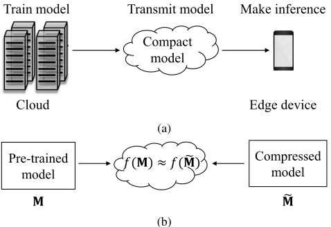
Figure 1: (a): In practice, a popular approach is to train a complete model for LMLL data with the usage of powerful computational platform, and then compress the model which is transmitted to edge devices to make inference. (b): The main difficulty in model compression is to retain a compara-ble performance while achieving a highly compressed model. Functionf measures the performance of the model.

the aspect of label space, data sets with thousands of labels have widely appeared in domains like object recognition and text classification (Zubiaga 2012).

The high dimensionality in both the feature and label spaces significantly increases the memory storage require-ments, limiting the deployment of LMLL algorithms in real-world applications (Prabhu and Varma 2014). For example, many effective approaches of traditional multi-label learning, such as the popular binary relevance scheme (Tsoumakas, Katakis, and Vlahavas 2009; Zhang and Zhou 2014; Babbar and Sch¨olkopf 2017; 2018), are hard to deal with modern LMLL data sets, since they have to systematically train a binary classifier for each label and thus the storage overhead scales linear to the number of features and labels, which is very expensive.

sig-𝑴𝑴

_𝑴𝑴

�

Label parameter

optimization Feature parameteroptimization

Model parameter Pruned label parameter Pruned feature parameter

Feature 1 Feature 2

Feature 𝑑𝑑 …

L

ab

el

1

L

ab

el

2

…

L

ab

el

𝐿𝐿

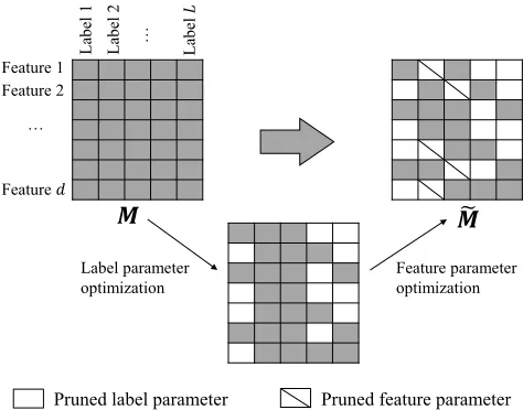
Figure 2: An illustration of our method. Given a pre-trained modelM, we perform joint label and feature parameter opti-mization to facilitate a compact modelM˜.

nificantly losing predictive performance (as demonstrated in Figure 1a and Figure 1b). We illustrate the proposed model compression method in Figure 2.

• In terms of label parameter optimization, ideally the most influential label parameters in terms of LMLL metrics (PSP@kand PSnDCG@k) are detected to facilitate com-pact models, which unfortunately is a hard optimization problem. Alternatively, we propose to detect the influential labels by calculating the performance impact for com-monly used LMLL metrics. The analyses show that the performance impact of labels is closely related to the la-bel importance and lala-bel frequency. Therefore, we only preserve a small number of dominant parameters for the labels that have little performance impact, which facilitates the compactness and retains a comparable performance.

• In terms of feature parameter optimization, since the most discriminative information is usually carried by only a sub-set of relevant features (Liu and Motoda 2007), we elim-inate the noisy, redundant and irrelevant features which marginally affect the learning performance. Specifically, the spurious feature parameters which have little contribu-tion to the generalizacontribu-tion capability are removed, so that the model size is shrunk.

Generally, we formulate the above aspects as a constrained optimization problem pursuing minimal model size. In order to solve the resultant difficult optimization, we show that a relaxation of the optimization can be efficiently solved using binary search and greedy strategies. Experiments verify that the proposed method clearly reduces the model size compared to state-of-the-art LMLL approaches, in addition, achieves highly competitive performance.

In the following, we first introduce related work and the commonly used LMLL performance metrics, and then we present the POPmethod, with the experimental results. Fi-nally we conclude this work.

Related Work

This work is mostly related to three branches of studies.

LMLL Model Compression Previous studies on LMLL model compression typically work on embedding approaches that project label vectors onto a low dimensional space based on the assumption that the label matrix is low-rank (Chen and Lin 2012; Kapoor, Viswanathan, and Jain 2012; Lin et al. 2014; Xu, Tao, and Xu 2016; Yeh et al. 2017). However, these studies do not take the pre-trained ‘optimal’ model into account and may lead to suboptimal performance. Recently, there are a few studies that yield a sparse version of the pre-trained ‘optimal’ model by filtering out spurious features parameters (Babbar and Sch¨olkopf 2017). However, they assume that all the labels are equally important, which may be not the case for LMLL performance metrics.

LMLL Feature Selection There are some studies about multi-label feature selection. For example, Zhang, Pe˜na, and Robles (2009) adapted the classical naive Bayes classifiers. Ma et al. (2012) proposed to learn a feature subspace that is shared among multiple different classes. Jian et al. (2016) introduced a principled way of exploiting label correlations for feature selection in the presence of noisy and incomplete label information. All these studies assume that features are useful or useless for all labels. In many cases, however, one feature which is useless to some labels may be critical to some others. Direct multi-label feature selection typically obtains a suboptimal solution.

LMLL Label Selection There are also some proposals on label selection in LMLL. For example, Boutsidis, Mahoney, and Drineas (2009) proposed to find approximate solutions of the column subset selection problem efficiently. Bi and Kwok (2013) selected a small subset of labels that can ap-proximately span the original label space. Weston, Makadia, and Yee (2013) partitioned the input space so that any given example can be mapped to a partition or set of partitions. Recently, Niculescu-Mizil and Abbasnejad (2017) proposed a label filter method to reduce prediction time. Different from above label selection methods, our proposal does not remove any label so that it can make predictions for all labels.

To our best knowledge, this paper is the first proposal on both label and feature parameter optimization for LMLL model compression.

Common Performance Metrics in LMLL

In this section, we introduce two commonly used LMLL performance metrics, PSP@kand PSnDCG@k(Babbar and Sch¨olkopf 2018; Jain, Prabhu, and Varma 2016).

PSP@k The first one is Propensity Scored Precision@k (PSP@k) proposed in (Jain, Prabhu, and Varma 2016). PSP@kis popularly used in LMLL applications, especially for ranking tasks such as information retrieval. In PSP@k, only a few top predictions of an instance will be considered. For instancex∈_Rd_{wheredrepresents the feature}

ˆ

y∈RLand ground truth label vectory∈ {0,1}Las

PSP@k(y,yˆ) := 1 k

X

l∈rankk(ˆy) yl

pl

where L is the size of label set and rankk(ˆy)returns the

indices ofklargest value inyˆ ranked in descending order. pl= _1+C(N1

l+B)−A is the propensity score for thel-th label,

whereA,B,Care set in a heuristic manner on different data sets andNlis the number of the positive training instances.

PSnDCG@k Propensity Scored nDCG@k(PSnDCG@k) is another commonly used ranking based performance mea-sure in LMLL and is defined as

PSnDCG@k(y,yˆ) := PSDCG@k

Pmin(k,||y||0) l=1

1 log(l+1)

where PSDCG@k(y,yˆ) := X

l∈rankk(ˆy) yl

pllog(l+ 1)

In particular, when settingpl = 1to all labels, PSP@k

and PSnDCG@kreduce to another two popular LMLL per-formance metrics P@kand nDCG@k, respectively.

Joint Label and Feature Parameter

Optimization (P

)

In this section, we present the proposed framework POP. Given a pre-trained LMLL model, our goal is to minimize the model size while retaining a comparable performance with the pre-trained LMLL model.

Formally, given the pre-trained modelM∈Rd×Land a set ofN samplesD={(xi,yi)}Ni=1wherexi ∈Rd,yi ∈

{0,1}L_{, the goal is to find a compact modelM˜ with}

compa-rable performance. Such objective can be formalized as,

min ˜

M

size( ˜M) (1)

s.t. f( ˜M,D)≥q∗−

where size( ˜M)returns the model size ofM˜,q∗ is the per-formance of modelMonD,controls the tolerance to per-formance deterioration, and functionf measures the perfor-mance of modelM˜ on dataD. In this paper, the pre-trained modelMis realized by binary relevance approaches shown state-of-the-art performance (Babbar and Sch¨olkopf 2017; 2018; Niculescu-Mizil and Abbasnejad 2017).

More specifically, by formulating the model size ofM˜ as

||_M˜_{||0andf( ˜M,D) = perf(XM}˜_{,Y), whereperf refers to}

commonly used LMLL performance metrics, i.e., PSP@k and PSnDCG@k. Eq. (1) can be reformulated as

min ˜

M

||M˜||0 (2)

s.t. perf(XM˜,Y)≥q∗−

However, the resultant optimization problem in Eq. (2) is difficult due to non-smoothness and non-convexity (Weston et al. 2003). To conquer the resultant difficult optimization, we propose to solve a relaxation of the problem, from label and feature parameter optimization aspects jointly.

Parameter Optimization w.r.t. Label

When optimizing label parameter, ideally the most influential labels with respect to LMLL metrics are located, meanwhile, the model does not lose the predictive capability for the remaining labels. Such ideal situation can be cast as the following form,

min ˜

M

L X

j=1

k

˜

M:,jk0−δ

₀ (3)

s.t. perf(XM˜,Y)≥q∗−

||M˜:,j||0≥δ, j = 1, . . . , L

whereM˜:,j indicates the j-th column of M˜, which

corre-sponds to the parameters for thej-th label, andδis a small constant indicating the least number of parameters need to be preserved for each label. From Eq. (3), we maintain the predictive capability for each label and meanwhile minimize the number of performance-influential labels.

Eq. (3), however, is a difficult integer programming prob-lem. Note that Eq. (3) can be viewed as selecting the most performance-influential labels. Following such intuition, we present to compute the performance impact of labels in terms of LMLL metrics so as to derive an approximate solution.

To capture the performance impact of labels, we study how labels affect the LMLL metrics under these two scenarios, i.e., missing labels and misclassified labels. The analysis shows that the performance impact of labels is proportional to its weight in LMLL metrics and its frequency in the observed data, which consequently provides a guideline to select the most influential labels.

Randomly Missing Labels Missing labels are commonly occurred in LMLL (Bi and Kwok 2013; Lin et al. 2014; Xu, Tao, and Xu 2016). In this section, we formally cap-ture the impact of labels under the missing labels scenario, that is,relevant labels are randomly missing with a

proba-bilityπ(Lim, McAuley, and Lanckriet 2015). Without loss

of generality, we letuj=||Y:,j||0(j= 1, ..., L)denote the

number of instances that have thej-th label. We usewj =p1j

to denote the weight for thej-th label, andciindicating the

number of relevant labels for instancexi.

Theorem 1. Suppose that relevant labels are randomly

miss-ing with probabilityπ, the impact of thej-th label in terms of

PSP@kand PSnDCG@kis upper bounded by(1−π)wjuj.

Proof. For PSP@k, sincekofcirelevant labels are selected

in the calculation of PSP@k, we have ci

k

distinct ways. The expected influence of thej-th label is computed as,

wj

k

N

X

i=1∧Yij=1 ci−1

k−1

ci k

= (1−)

N

X

i=1∧Yij=1

wj

ci

≤(1−π)wjuj

It can be seen that the impact of the j-th label is upper bounded by the product of label weightwj, its frequency

ujand a constant.

For PSnDCG@k, note that every observed label has the same rank, hence r = 1

constant and we have

PSnDCG@k= PSDCG@k

Pmin(k,kyk0) l=1

1 log(l+1)

= r

Pmin(k,kyk0)

l=1 r

X

l∈rankk(ˆy) yl

Since L is large in LMLL and k ≤ 5, we usually have ||y||0≥kand PSnDCG@kis cast as follows.

PSnDCG@k= _Pkr

l=1r

X

l∈rankk(ˆy) yl

= 1

k

X

l∈rankk(ˆy)

yl=PSP@k

As a result, the analysis for PSnDCG@kis reduced to the one in PSP@k.

Randomly Misclassified Labels Another common sce-nario is label misclassification (Schapire 1990; Wei and Li 2018). We also compute the impact of labels under the mis-classified label scenario, that is,labels are randomly

misclas-sified with probabilityπ.

Theorem 2. Suppose that labels are randomly misclassified

with probabilityπ, the impact of thej-th label on PSP@k

and PSnDCG@kis upper bounded by_(L(1−₋₂₎π_π)₊₁wjuj.

Proof. For PSP@k, there arevi = (1−π)ci+π(L−ci)

relevant labels in the predicted label vector. By choosing a random subset of sizekfromvilabels, the influence of the

j-th label to PSP@kcan be computed as

wj

k

N X

i=1∧Yij=1

vi−1

k−1

vi

k =

N X

i=1∧Yij=1

wj

vi

≤ (1−π)wjuj

(L−2)π+ 1 (4)

Eq. (4) shows that the influence of thej-th label is upper bounded by _(L(1−₋₂₎π_π)₊₁wjuj.

For PSnDCG@k, similar with the proof in Theorem 1, the proof for PSnDCG@kis reduced to the one in PSP@k, and we obtain same conclusive remark for PSnDCG@k.

According to the analyses, in both missing and label-misclassified scenarios, we find that impact of labels in terms of commonly LMLL metrics (PSP@kand PSnDCG@k) is proportional to the product of label weights and label frequen-cies. Therefore, we rank the labels according to the value of wjuj,j ={1, . . . , L}in ascending order, and filter out

pa-rameters for labels with little performance-impact. Due to the large number of labels, it is expensive to remove param-eters label by label until the constraint is violated. To this end, a binary search is developed to efficiently determine the threshold based on the observation that the performance is monotonically decreasing as the number of removed label parameters increases. By doing this, the computational cost is reduced fromO(L)toO(logL). Algorithm 1 summarizes the detailed procedure of binary search for label parameter optimization.

Parameter Optimization w.r.t. Feature

We further locate the most important feature parameters for the influential labels detected from label parameter optimiza-tion, and consequently remove spurious feature parameters to facilitate a compact model. Considering that Eq. (2) is difficult to solve due to non-smoothness and non-convexity, to this end, we propose to solve a relaxation of Eq. (2),

min ˜

M

||Y˜ −Y∗||2

F+λ||M˜||0 (5)

s.t. Y˜ =XM˜;Y∗=XM

where the constraintperf(XM˜,Y) ≥ q∗ −in Eq. (2) is relaxed as ||Y−Y∗||2

F, which encourages the predicted

label matrixY˜ ofM˜ andY∗from the pre-trained modelM to be closely related. The second term in Eq. (5) minimizes the number of non-zero entries inM˜, and the hyper-parameter λ >0trades off the predictive accuracy and the model size. The above optimization is difficult to solve. Inspired by (Zhao and Yu 2006), an approximate solution can be obtained by setting feature parameters that lie in range [−√λ,√λ]to 0. The closed-form approximation is based on the observation that each time a model parameter is weeded out, the termλ||M˜||0decreases byλirrespective of its value. Meanwhile, to minimize the reconstruction error||Y−Y∗||2

F,

we filter out model parameters starting from the entries with small absolute values to entries with large absolute values. The procedure terminates when the absolute value of the en-try that is to be removed in the next round is greater than√λ, which results in an increase to the objective. The pseudocode of the POPalgorithm is summarized in Algorithm 2.

Algorithm 1labelOptimization

Input: modelM; dataD; parameters,q∗,δ Output: compressed modelM˜

1: lowerBound = 0, upperBound = L 2: whileupperBound - lowerBound>1do 3: middle = (lowerBound + upperBound) / 2 4: M˜ =M

5: preserveδparameters with the largest absolute values inM˜:,j for thej-th label,j= 1, . . . ,middle

6: ifperf(XM˜,Y)≥q∗−then 7: lowerBound = middle 8: else

9: upperBound = middle 10: end if

11: end while

Experiments

We carry out extensive experiments on LMLL benchmark data sets to evaluate the effectiveness of our proposal.

Experimental Setup

Algorithm 2POP

Input: dataD; hyper-parameters,λ,δ Output: compact modelM˜

1: sort labels according towjuj,j={1, . . . , L}in

ascend-ing order

2: train LMLL modelMand obtain its performanceq∗ 3: M˜ = labelOptimization(M,D,,q∗,δ)

4: set entries ofM˜ in range[−√λ,√λ]to 0 and at leastδ parameters preserved for each label

and wiki10 (web page categorization, 30K labels). We re-port and compare the results using the same train/test splits of data sets. All the data sets as well as the experimental results of state-of-the-art LMLL methods are publicly avail-able, and can be downloaded from the Extreme Classification Repository1_.

Compared Methods We compare our method to Binary Relevance (BR) and six state-of-the-art LMLL baselines. • Binary Relevance (Zhang and Zhou 2014) builds

one-vs-all SVM for each label using Liblinear (Fan et al. 2008). • LEML (Yu et al. 2014) is an embedding method based on

low-rank empirical risk minimization.

• FastXML (Prabhu and Varma 2014) is a random forest based LMLL approach.

• SLEEC (Bhatia et al. 2015) learns the embedding of labels by preserving the pairwise distances between a few nearest label neighbors.

• CoH (Shen et al. 2018) proposes a co-hashing method which jointly compresses the input and output into compact binary embeddings.

• DisMEC (Babbar and Sch¨olkopf 2017) learns a 1vsA linear-SVM in a distributed fashion.

• PD-Sparse (Yen et al. 2016) proposes to solveL1 regular-ized multi-class loss using Frank-Wolfe based algorithm.

We use BR as the base classifier and build POPbased on it.

Hyper-parameters In all of our experiments, we fix the least number of preserved label parametersδto 5. For LEML, FastXML, SLEEC, and CoH, we use the default parameter settings in the code.

Computational Device All experimental comparisons are conducted on a same PC machine with an Intel i5-6500 3.20GHz CPU and 32GB RAM.

P

vs. Uncompressed Baseline

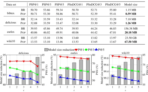
We first study how effective POPis at reducing the model size in comparison with plain BR. The comparison results with the plain binary relevance approach are depicted in Table 1. On relatively small data set bibtex, POPimproves above 50% model size and loses no more than 0.5% performance in terms of six different metrics. Considering the relatively balanced label distribution due to the small label set and hence only a

1

http://manikvarma.org/downloads/XC/XMLRepository.html

few label parameters can be pruned, otherwise resulting in serious performance deterioration. On the other three larger data sets with high dimensionality of feature and label space, the model size is improved by more than 80%. As a result, we obtain a significant reduction in model size with highly comparable generalization performance.

P

vs. Compressed Baselines

We further compare the performance of POP with DiS-MEC and PD-Saprse. We report the result from the Extreme Classification Repository in Table 2. DiSMEC reduces the model size by pruning spurious feature parameters as a post-processing step, which can be viewed as a subprocedure of POP. In terms of PSP@k and PSnDCG@k, DiSMEC achieves similar performance with our method. However, for model size, POPleads to as much as10x reduction on wiki10 and about4x reduction on eurlex, which shows the merit of our proposal. For PD-Sparse, due to its linear nature, its model size is small, but predictive accuracy is also limited by the capacity of the model. For instance, POPgets more than 5% better performance than PD-Sparse in most cases. The result shows that POPfinds a proper balance between model capacity and predictive accuracy.

P

vs. State-of-the-art Methods

In this experiment, we compare the performance of POPwith state-of-the-art methods: FastXML, LEML, SLEEC, and CoH. As demonstrated in Table 2, although POPis built on the binary relevance scheme, it achieves comparable or even smaller model size compared to state-of-the-art approaches. However, in terms of predictive performance, solvers relied on structural assumptions such as FastXML (tree), LEML (low-rank), SLEEC (piecewise-low-rank) do not perform as well as POPin most cases. This may owe to the fact that low-rank or tree assumption does not exactly hold in these data sets. On the aspect of model size, we can see that POPgets an order of magnitude smaller model size than FastXML and SLEEC. Compared with CoH, we achieve better performance with a large margin on all data sets and a smaller model size in most cases.

Parameter Sensitivities Analysis

We further investigate the influence ofandλto the perfor-mance of POP.

Impact of We study how different values ofimpact the predictive accuracy and model size. Figure 3 demonstrates that performance deteriorates as the value ofgrows because it determines the fraction of removed parameters for labels and in return, hurts the performance when informative label parameters are pruned. On the aspect of model size, POPis able to filter out more than 80% model parameters even when= 1%. Although more significant reduction can be gained with a larger value of, it comes at the cost of losing generalization accuracy.

Table 1: Performance comparison between the proposed POPmethod and BR in terms of PSP@k(%), PSnDCG@k(%), and Model size withλ= 0.01 and= 1%. The best results in terms of model size are in bold.

Data set PSP@1 PSP@3 PSP@5 PSnDCG@1 PSnDCG@3 PSnDCG@5 Model size

bibtex

BR 50.70 53.66 59.34 50.70 52.71 55.80 1.15 MB

POP 50.71 53.30 58.86 50.71 52.39 55.41 0.59 MB

delicious

BR 32.14 33.59 33.43 32.14 33.32 33.28 7.18 MB

POP 32.08 33.59 33.47 32.08 33.30 33.29 1.26 MB

eurlex

BR 39.93 45.86 49.74 39.93 44.24 46.83 156.38 MB

POP 40.06 46.02 49.91 40.06 44.42 47.01 20.18 MB

wiki10

BR 13.57 13.10 13.96 13.60 13.82 13.97 23.50 GB

POP 13.53 13.10 13.46 13.53 13.65 13.67 67.50 MB

0.01 0.03 0.05 0.07 0.09

6

20

30

40

50

60

70

80

Model size reduction (%)

bibtex

25

35

45

55

65

P@

k

(%)

Model size reduction P@1 P@3 P@5

1 2 3 4 5

0

80 85 90 95

Model size reduction (%)

delicious

45 50 55 60 65

P@

k

(%)

1 2 3 4 5

0

85 90 95

Model size reduction (%)

eurlex

50 60 70 80

P@

k

(%)

1 2 3 4 5

0 99

99.2 99.4 99.6 99.8

Model size reduction (%)

wiki10

55 65 75 85

P@

k

(%)

Figure 3: Study on different value ofwithλset to 0.01. X-axis: value of(%). Y-axis (Left): percentage of model size reduction compared to the plain BR. Y-axis (Right): P@k.

0.01 0.03 0.05 0.07 0.09

6

20

30

40

50

60

70

80

Model size reduction (%)

bibtex

25

35

45

55

65

P@

k

(%)

Model size reduction P@1 P@3 P@5

0.01 0.03 0.05 0.07 0.09 6

80 82 84 86

Model size reduction (%)

delicious

50 55 60

P@

k

(%)

0.01 0.03 0.05 0.07 0.09 6

85 90 95 100

Model size reduction (%)

eurlex

40 50 60 70 80

P@

k

(%)

0.01 0.03 0.05 0.07 0.09 6

99 99.2 99.4 99.6 99.8 100

Model size reduction (%)

wiki10

35 45 55 65 75 85

P@

k

(%)

Figure 4: Study on different value ofλwithset to 1%. X-axis: value ofλ. Y-axis (Left): percentage of model size reduction compared to the plain BR. Y-axis (Right): P@k.

small, the model size is reduced by at least 80%. As the value ofλslightly grows, the performance does not affect. How-ever, when too large values ofλare used, the model becomes excessively sparse and many discriminative parameters are wrongly eliminated, deteriorating performance. Our empiri-cal results show that POPperforms well in a wide range of,

but is relatively sensitive toλon some data sets.

Conclusion

Table 2: Comparison with state-of-the-art approaches in terms of model size, PSP@k(%) and PSnDCG@k(%). Results for CoH are partially available due to the high computational cost. The best and the second best results are in bold.

Data set FastXML LEML SLEEC CoH DiSMEC PD-Sparse POP(ours)

bibtex

Model size 18.72 MB 0.76 MB 2.46 MB 4.70 MB 0.71 MB 20.00 KB 0.59 MB

PSP@1 48.54 47.97 51.12 36.53 50.20 48.34 50.71

PSP@3 52.30 51.42 53.95 28.20 52.20 48.77 53.30

PSP@5 58.28 57.53 59.56 25.59 58.60 52.93 58.86

PSnDCG@1 48.54 47.97 51.12 36.58 50.20 48.34 50.71

PSnDCG@3 51.11 50.25 52.99 30.62 52.00 48.49 52.39

PSnDCG@5 54.38 53.59 56.04 29.06 55.70 50.72 55.41

delicious

Model size 71.29 MB 2.26 MB 7.34 MB 10.92 MB - 0.25 MB 1.26 MB

PSP@1 32.35 30.73 32.11 20.43 - 25.22 32.08

PSP@3 34.51 32.43 33.21 22.76 - 24.63 33.59

PSP@5 35.43 33.26 33.83 24.11 - 23.85 33.47

PSnDCG@1 32.35 30.73 32.11 20.43 - 25.22 32.08

PSnDCG@3 34.00 32.01 32.93 22.16 - 24.80 33.30

PSnDCG@5 34.73 32.66 33.41 23.20 - 24.25 33.29

eurlex

Model size 194.40 MB 34.31 MB 245.49 MB 15.95 MB 79.86 MB 25.00 MB 20.18 MB

PSP@1 26.62 24.10 34.25 20.78 41.20 38.28 40.06

PSP@3 34.16 27.20 39.83 22.98 45.40 42.00 46.02

PSP@5 38.96 29.09 42.76 21.89 49.30 44.89 49.91

PSnDCG@1 26.62 24.10 34.25 20.78 41.20 38.28 40.06

PSnDCG@3 32.07 26.37 38.35 22.49 44.30 40.96 43.55

PSnDCG@5 35.23 27.62 40.30 21.92 46.90 42.84 47.01

wiki10

Model size 501.47 MB 506.88 MB 924.60 MB - 880.00 MB - 67.50 MB

PSP@1 9.80 9.41 11.14 - 13.60 - 13.53

PSP@3 10.17 10.07 11.86 - 13.10 - 13.10

PSP@5 10.54 10.55 12.40 - 13.80 - 13.46

PSnDCG@1 9.80 9.41 11.14 - 13.60 - 13.53

PSnDCG@3 10.08 9.90 11.68 - 13.20 - 13.65

PSnDCG@5 10.33 10.24 12.06 - 13.60 - 13.67

parameters which have little impact on the predictive accu-racy, as well as to prune redundant feature parameters. We formulate this as a constrained optimizing problem and solve its relaxation form effectively with binary search and greedy strategies. Empirical results demonstrate that the proposed method is capable of reducing the model size, in addition, achieves highly competitive performance. In future, we will study how to improve the performance on few relevant in-stances (Wei et al. 2018) and derive LMLL models with both high performance and lightweight storage.

Acknowledgments

This research was supported by the National Key R&D Pro-gram of China (2017YFB1001903) and the National Natural Science Foundation of China (61772262). Yu-Feng Li is the corresponding author. We also would like to thank Wei-Wei Tu and Hai Wang for helpful discussions.

References

Abu-El-Haija, S.; Kothari, N.; Lee, J.; Natsev, P.; Toderici, G.; Varadarajan, B.; and Vijayanarasimhan, S. 2016. Youtube-8m: A large-scale video classification benchmark. arXiv

preprint arXiv:1609.08675.

Babbar, R., and Sch¨olkopf, B. 2017. Dismec: Distributed sparse machines for extreme multi-label classification. In

Proceedings of the 10th ACM International Conference on

Web Search and Data Mining, 721–729.

Babbar, R., and Sch¨olkopf, B. 2018. Adversarial extreme multi-label classification. arXiv preprint arXiv:1803.01570. Bhatia, K.; Jain, H.; Kar, P.; Varma, M.; and Jbabain, P. 2015. Sparse local embeddings for extreme multi-label classifica-tion. InAdvances in Neural Information Processing Systems 28. 730–738.

classifi-cation with many labels. InProceedings of the 30th

Interna-tional Conference on Machine Learning, 405–413.

Boutsidis, C.; Mahoney, M. W.; and Drineas, P. 2009. An improved approximation algorithm for the column subset selection problem. InProceedings of the 20th annual

ACM-SIAM symposium on Discrete algorithms, 968–977.

Chen, Y.-N., and Lin, H.-T. 2012. Feature-aware label space dimension reduction for multi-label classification. In

Ad-vances in Neural Information Processing Systems 25. 1529–

1537.

Deng, J.; Dong, W.; Socher, R.; Li, L.-J.; Li, K.; and F.-F., L. 2009. Imagenet: A large-scale hierarchical image database.

InProceedings of the 22nd IEEE Conference on Computer

Vision and Pattern Recognition, 248–255.

Fan, R.-E.; Chang, K.-W.; Hsieh, C.-J.; Wang, X.-R.; and Lin, C.-J. 2008. Liblinear: A library for large linear classification.

Journal of Machine Learning Research9:1871–1874.

Jain, H.; Prabhu, Y.; and Varma, M. 2016. Extreme multi-label loss functions for recommendation, tagging, ranking & other missing label applications. InProceedings of the 22nd ACM SIGKDD International Conference on Knowledge

Discovery and Data Mining, 935–944.

Jian, L.; Li, J.-D.; Shu, K.; and Liu, H. 2016. Multi-label informed feature selection. InProceedings of the 25th

In-ternational Joint Conference on Artificial Intelligence, 1627–

1633.

Kapoor, A.; Viswanathan, R.; and Jain, P. 2012. Multilabel classification using bayesian compressed sensing. In

Ad-vances in Neural Information Processing Systems 25. 2645–

2653.

Lim, D.; McAuley, J.; and Lanckriet, G. 2015. Top-n recom-mendation with missing implicit feedback. InProceedings

of the 9th ACM Conference on Recommender Systems, 309–

312.

Lin, Z.-J.; Ding, G.-G.; Hu, M.-Q.; and Wang, J.-M. 2014. Multi-label classification via feature-aware implicit label space encoding. InProceedings of the 31st International

Conference on Machine Learning, 325–333.

Liu, H., and Motoda, H. 2007. Computational methods of

feature selection. CRC Press.

Ma, Z.-G.; Nie, F.-P.; Yang, Y.; Uijlings, J. R.; and Sebe, N. 2012. Web image annotation via subspace-sparsity collab-orated feature selection.IEEE Transactions on Multimedia

14(4):1021–1030.

McAuley, J.; Pandey, R.; and Leskovec, J. 2015. Inferring networks of substitutable and complementary products. In

Proceedings of the 21th ACM SIGKDD International

Confer-ence on Knowledge Discovery and Data Mining, 785–794.

Niculescu-Mizil, A., and Abbasnejad, M. E. 2017. Label fil-ters for large scale multi-label classification. InProceedings of the 20th International Conference on Artificial Intelligence

and Statistics, 1448–1457.

Partalas, I.; Kosmopoulos, A.; Baskiotis, N.; Artieres, T.; Paliouras, G.; Gaussier, E.; Androutsopoulos, I.; Amini, M.-R.; and Galinari, P. 2015. Lshtc: A benchmark for large-scale text classification.arXiv preprint arXiv:1503.08581.

Prabhu, Y., and Varma, M. 2014. Fastxml: A fast, accurate and stable tree-classifier for extreme multi-label learning. In

Proceedings of the 20th ACM SIGKDD International

Confer-ence on Knowledge Discovery and Data Mining, 263–272.

Schapire, R. E. 1990. The strength of weak learnability.

Machine Learning5(2):197–227.

Shen, X.; Liu, W.; Tsang, I. W.; Sun, Q.-S.; and Ong, Y.-S. 2018. Compact multi-label learning. InProceedings of the

32nd AAAI Conference on Artificial Intelligence, 4066–4073.

Tsoumakas, G.; Katakis, I.; and Vlahavas, I. 2009. Mining multi-label data. InData Mining and Knowledge Discovery

handbook. Springer. 667–685.

Wei, T., and Li, Y.-F. 2018. Does tail label help for large-scale multi-label learning. InProceedings of the 27th International

Joint Conference on Artificial Intelligence, 2847–2853.

Wei, T.; Guo, L.-Z.; Li, Y.-F.; and Gao, W. 2018. Learning safe multi-label prediction for weakly labeled data. Machine

Learning107(4):703–725.

Weston, J.; Elisseeff, A.; Sch¨olkopf, B.; and Tipping, M. 2003. Use of the zero-norm with linear models and kernel methods. Journal of Machine Learning Research3:1439– 1461.

Weston, J.; Makadia, A.; and Yee, H. 2013. Label parti-tioning for sublinear ranking. InProceedings of the 30th

International Conference on Machine Learning, 181–189.

Xu, C.; Tao, D.-C.; and Xu, C. 2016. Robust extreme multi-label learning. InProceedings of the 22nd ACM SIGKDD International Conference on Knowledge Discovery and Data

Mining, 1275–1284.

Yeh, C.-K.; Wu, W.-C.; Ko, W.-J.; and Wang, Y.-C. F. 2017. Learning deep latent space for multi-label classification. In

Proceedings of the 31st AAAI Conference on Artificial

Intelli-gence, 2838–2844.

Yen, I. E.-H.; Huang, X.-R.; Ravikumar, P.; Zhong, K.; and Dhillon, I. S. 2016. Pd-sparse: A primal and dual sparse approach to extreme multiclass and multilabel classification.

InProceedings of the 33rd International Conference on

Ma-chine Learning, 3069–3077.

Yu, H.-F.; Jain, P.; Kar, P.; and Dhillon, I. S. 2014. Large-scale multi-label learning with missing labels. InProceedings

of the 31st International Conference on Machine Learning,

593–601.

Zhang, M.-L., and Zhou, Z.-H. 2014. A review on multi-label learning algorithms.IEEE Transactions on Knowledge and

Data Engineering26(8):1819–1837.

Zhang, M.-L.; Pe˜na, J. M.; and Robles, V. 2009. Feature se-lection for multi-label naive bayes classification.Information

Sciences179(19):3218–3229.