The Thirty-Third AAAI Conference on Artificial Intelligence (AAAI-19)
How to Combine Tree-Search Methods in Reinforcement Learning
Yonathan Efroni
Technion, IsraelGal Dalal
Technion, IsraelBruno Scherrer
INRIA, Villers les Nancy, FranceShie Mannor
Technion, IsraelAbstract
Finite-horizon lookahead policies are abundantly used in Re-inforcement Learning and demonstrate impressive empirical success. Usually, the lookahead policies are implemented with specific planning methods such as Monte Carlo Tree Search (e.g. in AlphaZero (Silver et al. 2017b)). Referring to the plan-ning problem as tree search, a reasonable practice in these im-plementations is to back up the value only at the leaves while the information obtained at the root is not leveraged other than for updating the policy. Here, we question the potency of this approach. Namely, the latter procedure is non-contractive in general, and its convergence is not guaranteed. Our proposed enhancement is straightforward and simple: use the return from the optimal tree path to back up the values at the descen-dants of the root. This leads to aγh
-contracting procedure, whereγis the discount factor andhis the tree depth. To estab-lish our results, we first introduce a notion calledmultiple-step greedy consistency. We then provide convergence rates for two algorithmic instantiations of the above enhancement in the presence of noise injected to both the tree search stage and value estimation stage.
1
Introduction
A significant portion of the Reinforcement Learning (RL) literature regards Policy Iteration (PI) methods. This fam-ily of algorithms contains numerous variants which were thoroughly analyzed (Puterman 1994; Bertsekas and Tsit-siklis 1995) and constitute the foundation of sophisticated state-of-the-art implementations (Mnih et al. 2016; Silver et al. 2017b). The principal mechanism of PI is to alternate between policy evaluation and policy improvement. Vari-ous well-studied approaches exist for the policy evaluation stages; these may rely on single-step bootstrap, multi-step Monte-Carlo return, or parameter-controlled interpolation of the former two. For the policy improvement stage, theoreti-cal analysis was mostly reserved for policies that are 1-step greedy, while recent prominent implementations of multiple-step greedy policies exhibited promising empirical behavior (Silver et al. 2017b; 2017a).
Relying on recent advances in the analysis of multiple-step lookahead policies (Efroni et al. 2018a; 2018c), we study the convergence of a PI scheme whose improvement stage is
Copyright c2019, Association for the Advancement of Artificial Intelligence (www.aaai.org). All rights reserved.
h-step greedy with respect to (w.r.t.) the value function, for
h >1.Calculating such policies can be done via Dynamic Programming (DP) or other planning methods such as tree search. Combined with sampling, the latter corresponds to the famous Monte Carlo Tree Search (MCTS) algorithm employed in (Silver et al. 2017b; 2017a). In this work, we show that even when partial (inexact) policy evaluation is performed and noise is added to it, along with a noisy policy improvement stage, the above PI scheme converges with a
γhcontraction coefficient. While doing so, we also isolate a sufficient convergence condition which we refer to ash -greedy consistencyand relate it to previous 1-step greedy relevant literature.
A straightforward ‘naive’ implementation of the PI scheme described above would perform anh-step greedy policy im-provement and then evaluate that policy by bootstrapping the ‘usual’ value function. Surprisingly, we find that this
proce-dure does not necessarily contracts toward the optimal value, and give an example where it is indeed non-contractive. This contraction coefficient depends both onhand on the partial evaluation parameter:min the case ofm-step return, and
λwhen eligibility trace is used. The non-contraction occurs even when theh-greedy consistency condition is satisfied.
To solve this issue, we propose an easy fix which we em-ploy in all our algorithms, that relieves the convergence rate from the dependence ofmandλ, and allows theγh
contrac-tion mencontrac-tioned earlier in this seccontrac-tion. Let us treat each state as a root of a tree of depthh;then our proposed fix is the fol-lowing. Instead of backing up the value only at the leaves and ridding of all non-root related tree-search outputs, we reuse the tree-search byproducts and back up the optimal value of the root node children. Hence, instead of bootstrapping the ‘usual’ value function in the evaluation stage, we bootstrap the optimal value obtained from theh−1horizon optimal planning problem.
over the alternative ‘naive’ approach. A more recent work (Lai 2015) introduced a deep learning implementation of TDLeaf(λ) called Giraffe. Testing it on the game of Chess, the authors claim (during publication) it is “the most success-ful attempt thus far at using end-to-end machine learning to play chess”. In light of our theoretical results and empirical success described above, we argue that backing up the opti-mal value from a tree search should be considered as a ‘best practice’ among RL practitioners.
2
Preliminaries
Our framework is the infinite-horizon discounted Markov Decision Process (MDP). An MDP is defined as the 5-tuple
(S,A, P, R, γ)(Puterman 1994), whereS is a finite state space,Ais a finite action space,P ≡P(s0|s, a)is a transi-tion kernel,R ≡r(s, a) ∈[Rmin, Rmax]is a reward
func-tion, andγ∈(0,1)is a discount factor. Letπ:S → P(A)
be a stationary policy, where P(A)is a probability distri-bution onA. Let vπ ∈ R|S| be the value of a policy π,
defined in state s as vπ(s) ≡ Eπ|s[
P∞ t=0γ
tr(s
t, π(st))],
where Eπ|s denotes expectation w.r.t. the distribution
in-duced by π and conditioned on the event {s0 = s}.
For brevity, we respectively denote the reward and value at time t by rt ≡ r(st, πt(st)) and vt ≡ v(st). It is
known thatvπ =P∞
t=0γt(Pπ)trπ= (I−γPπ)−1rπ, with
the component-wise values[Pπ]s,s0 ,P(s0 |s, π(s))and
[rπ]
s,r(s, π(s)). Our goal is to find a policyπ∗yielding
the optimal valuev∗such thatv∗ = max
π(I−γPπ)−1rπ.
This goal can be achieved using the three classical operators (with equalities holding component-wise):
∀v, π, Tπv=rπ+γPπv, (1)
∀v, T v= max
π T
π
v, (2)
∀v, G(v) ={π:Tπv=T v}, (3) where Tπ is a linear operator, T is the optimal Bellman operator and bothTπandTareγ-contraction mappings w.r.t.
the max norm. It is known that the unique fixed points ofTπ
andTarevπandv∗, respectively. The setG(v)is the standard
set of 1-step greedy policies w.r.t. v. Furthermore, given
v∗, the setG(v∗)coincides with that of stationary optimal policies. In other words, every policy that is 1-step greedy w.r.t.v∗is optimal and vice versa.
The most known variants of PI are Modified-PI (Puter-man and Shin 1978) andλ-PI (Bertsekas and Ioffe 1996). In both, the evaluation stage of PI is relaxed by performing partial-evaluation, instead of the full policy evaluation. In this work, we will generalize algorithms using both of these approaches. Modified PI performs partial evaluation using them-return,(Tπ)mv, whereλ-PI uses theλ-return,Tλπv, withλ∈[0,1]. This operator has the following equivalent forms (see e.g. (Scherrer 2013), p.1182),
Tλπv
def
= (1−λ)
∞
X
j=0
λj(Tπ)j+1v (4)
=v+ (I−γλPπ)−1(Tπv−v).
rt=0
γrt=1
γ2v
t=2
s
sr sl
Figure 1: Obtaining theh-greedy policy with a tree-search also outputs TπhTh−1v andTh−1v. In this example, the
red arrow depicts theh-greedy policy. The value at the root’s child nodeslisTh−1v(sl),which corresponds to the optimal
blue trajectory starting atsl. The same holds forsr.
These operators correspond to the ones used in the famous TD(n) and TD(λ) (Sutton, Barto, and others 1998),
(Tπ)mv=Eπ|• "m−1
X
t=0
γtr(st, πt(st)) +γmv(sh) #
,
Tλπv=v+Eπ|• "∞
X
t=0
(γλ)t(rt+γvt+1−vt) #
.
3
The
h
-Greedy Policy and
h
-PI
Leth∈N\{0}. Anh-greedy policy (Bertsekas and Tsitsiklis 1995; Efroni et al. 2018a)πhoutputs the first optimal actionout of the sequence of actions solving a non-stationary,h -horizon control problem as follows:
arg max
π0 max
π1,..,πh−1
Eπ|•0...πh−1
"h−1 X
t=0
γtr(st, πt(st)) +γhv(sh)
#
= arg max
π0 E
π0
|•
r(s0, π0(s0)) +γ Th−1v (s1)
, (5)
where the notation Eπ|•0...πh−1 corresponds to
condition-ing on the trajectory induced by the choice of actions
(π0(s0), π1(s1), . . . , πh−1(sh−1))and a starting states0=•.
As the equality in (5) suggests thatπhcan be interpreted
as a 1-step greedy policy w.r.t.Th−1v. We denote the set of h-greedy polices w.r.tvasGh(v)and is defined by
∀v, Gh(v) ={π:TπTh−1v=Thv}.
This generalizes the definition of the 1-step greedy set of policies, generalizing, (3), and coincides with it forh= 1. Remark 1. Theh-greedy policy can be obtained by solv-ing the above formulation with DP in linear time (in h). Other than returning the policy, the last and one-before-last iterations also returnTπhTh−1vandTh−1v,respectively. Another, conceptually similar option would be using Model Predictive Control to solve the planning problem and again retrieve the above values of interest (Negenborn et al. 2005; Tamar et al. 2017). Given a ‘nice’ mathematical structure, this can be done efficiently. When the model is unknown, find-ingπhtogether withTπhTh−1vandTh−1vis possible with
depthh, starting at roots(see Figure 1). The search again returnsTπhTh−1v andTh−1v “for free” as the values at the root and its descendant nodes. While the tree-search com-plexity in general is exponential inh, sampling can be used. Examples for such sampling-based tree-search methods are MCTS (Browne et al. 2012) and Optimistic Tree Exploration (Munos 2014).
Algorithm 1h-PI
Initialize:h∈N\ {0}, v0=vπ0 ∈R|S|
whilevkchangesdo πk ←π∈ Gh(v) vk+1←vπk
k ←k+ 1
end while Returnπ, v
As was discussed in (Bertsekas and Tsitsiklis 1995; Efroni et al. 2018a), one can use theh-greedy policy to derive a policy-iteration procedure calledh-PI (see Algorithm 1). In it, the 1-step greedy policy from PI is replaced with theh -greedy policy. This algorithm iteratively calculates anh-step greedy policy with respect tov, and then performs a complete evaluation of this policy. Convergence is guaranteed after
O(h−1)iterations (Efroni et al. 2018a).
4
h
-Greedy Consistency
Theh-greedy policy w.r.tvπ is strictly better thanπ, i.e., vπh ≥vπ(Bertsekas and Tsitsiklis 1995; Efroni et al. 2018a).
Using this property for proving convergence of an algorithm requires the algorithm to perform exact value estimation, which can be a hard task. Instead, in this work, we replace the less practical exact evaluation with partial evaluation; this comes with the price of more challenging analysis. Tackling this more intricate setup, we identify a key property required for the analysis to hold. We refer to it ash-greedy consistency. It will be central to all proofs in this work.
Definition 1. A pair of value function and policy(v, π)is h-greedy consistent ifTπTh−1v≥Th−1v.
In words,(v, π)ish-greedy consistent ifπ‘improves’, component-wise, the valueTh−1v. Since relaxing the
evalua-tion stage comes with theh-greedy consistency requirement, the following question arises: while dispatching an algorithm, what is the price ensuringh-greedy consistency per each it-eration? As we will see in the coming sections, it is enough to ensureh-greedy consistency only for the first iteration of our algorithms. For the rest of the iterations it holds by con-struction and is shown to be guaranteed in our proofs. Thus, by only initializing to anh-greedy consistent(v0, π0), we
enable guaranteeing the convergence of an algorithm that per-forms partial evaluation instead of exact in each its iterations. Ensuring consistency for the first iteration is straightforward, as is explained in the following remark.
Remark 2. Choosing(v, π)which ish-greedy consistent can be done, e.g., by choosingv= Rmin
1−γ (i.e., set every
en-trance ofvto the minimal possible accumulated reward) and
π=πh∈ Gh(v).Furthermore, for any value-policy,(¯v, π),
that is noth-greedy consistent, let
∆ = maxs T
h−1v¯−TπTh−1¯v
(s) γh−1(1−γ) >0,
and setv= ¯v−∆. Then,(v, π)ish-greedy consistent. This is a generalization to the construction given forh= 1(see (Bertsekas and Tsitsiklis 1995), p. 46).
h-greedy consistency is anh-step generalization of a no-tion already introduced in previous works on 1-step-based PI schemes with partial evaluation. The latter are known as ‘optimistic’ PI schemes and include Modified PI andλ-PI (Bertsekas and Tsitsiklis 1995). There, the initial value-policy pair is assumed to be 1-greedy consistent, i.e.Tπ1v
0 ≥v0,
e.g., (Bertsekas and Tsitsiklis 1995), p. 32 and 45, (Bertsekas 2011), p. 3, (Puterman and Shin 1978)[Theorem 2]. This property served as an assumption on the pair(v0, π1).
To further motivate our interest in Definition 1, in the rest of the section we give two results that would be used in proofs later but are also insightful on their own. The following lemma gives thath-greedy consistency implies a sequence of value-function partial evaluation relations (proof in (Efroni et al. 2018b)).
Lemma 1. Let(v, π)beh-greedy consistent. Then,
TπTh−1v≤ · · · ≤(Tπ)lTh−1v≤ · · · ≤vπ.
The result shows that vπ is strictly bigger thanTh−1v.
This property holds whenv =vπ0, i.e., whenvis an exact
value of some policy and was central in the analysis ofh-PI (Efroni et al. 2018a). However, as Lemma 1 suggests, we only needh-greedy consistency, which is easier to have than estimating the exact value of a policy (see Remark 2).
The next result shows that ifπis taken to be theh-greedy policy, using partial evaluation results in aγhcontraction
toward the optimal valuev∗(proof in (Efroni et al. 2018b)). Proposition 2. Let vandπh ∈ Gh(v)be s.t.(v, πh)ish
-greedy consistent. Then, for anym≥1andλ∈[0,1],
||v∗−(Tπh)mTh−1v||
∞≤γh||v∗−v||∞and
||v∗−Tπh
λ T
h−1v||
∞≤γh||v∗−v||∞.
In (Efroni et al. 2018a)[Lemma 2], a similar contraction property was proved and played a central role in the anal-ysis of the correspondingh-PI algorithm. Again, there, the requirement wasv=vπ0.Instead, the above result requires
a weaker condition:h-greedy consistency of(v, πh).
5
The
h
-Greedy Policy Alone is Not
Sufficient For Partial Evaluation
A more practical version ofh-PI (Algorithm 1) would involve them- orλ-return w.r.t.vkinstead of the exact value. Thiswould correspond to the update rules:
πk ←arg max
π T
πTh−1v
k, (6)
Indeed, this would relax the evaluation task to an easier task than full policy evaluation.
The next theorem suggests that forπh ∈ Gh(v),even if
(v, πh)ish-greedy consistent, the procedure (6)-(7) does not
necessarily contract toward the optimal policy, unlike the form of update in Proposition 2. To see that, note that both
γm+γhandγ1(1−−λγλ)+γhcan be larger than 1.
Theorem 3. Leth > 1, m ≥ 1, andλ ∈ [0,1]. Let vbe a value function andπh ∈ Gh(v)s.t.(v, πh) ish-greedy
consistent (see Definition 1). Then,
||v∗−(Tπh)mv||
∞≤(γm+γh)||v∗−v||∞, (8)
||v∗−Tπh λ v||∞≤
γ(1−λ) 1−λγ +γ
h
||v∗−v||∞. (9)
Additionally, there exist aγ-discounted MDP, value function v,and policyπh∈ Gh(v)s.t.(v, πh)ish-greedy consistent,
for which(8)and(9)hold with equality.
The proof of the first statement is given in (Efroni et al. 2018b), and the proof of the second statement is as follows.
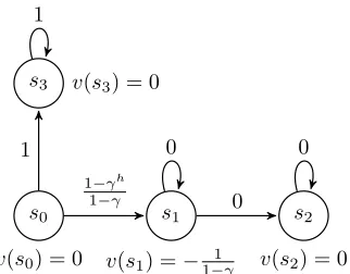
Proof of second statement in Theorem 3. We prove this by constructing an example. Fixh >1and consider the corre-sponding 4-state MDP in Figure 2. Letvbev(s0) =v(s2) = v(s3) = 0, v(s1) = − 1
1−γ. Also, let πh ∈ Gh(v). For
this choice, observe thatTh−1v≤TπhTh−1v, i.e.,(v, π h)
is h-greedy consistent. The optimal policy from state s0
is to choose the action ‘up’. Thus, it is easy to see that,
v∗(s0) =v∗(s3) = 1−1γ, and in the remaining of states it is easy to observe thatv∗(s1) =v∗(s2) = 0.
Now, see that for any h > 1 Th−1v(s1) = Th−1v(s2) = 0, Th−1v(s3) = 1−1γ−h−γ1. Thus, the
h-greedy policy (by using (5)) is contained in the fol-lowing set of actions πh(s0) ∈ {right,up}, πh(s1) ∈
{right,stay}, πh(s2), πh(s3) ∈ {stay}. For example, we
see that taking the action ‘stay’ or ‘right’ from states1and
then obtainTh−1vhave equal value: r(s1,‘stay0) +γ(Th−1v)(s1) =r(s1,‘right0) +γ(Th−1v)(s2) = 0.
Let us choose anh-greedy policy,πh, of the form:πh(s0) =
right, πh(s1) = stay, πh(s2) = stay.Thus, from states0,
them-return has the value
((Tπh)mv) (s
0) =
m−1
X
i=0
γtr(si, πh(si)) +γmv(si=m)
=1−γ
m−γh
1−γ +
m−1
X
i=1
γi·0 +γm
− 1
1−γ
=1−γ
m−γh
1−γ
We thus have that
||v∗−(Tπh)mv||∞=|v∗(s1,0)−(Tπh)mv(s1,0)|
= 1
1−γ +
γm+γh−1
1−γ = (γ
m+γh) 1
1−γ (10)
s0
v(s0) = 0
s1
v(s1) =− 1 1−γ
s2
v(s2) = 0 s3 v(s3) = 0
1−γh
1−γ 0
0 1
1 0
Figure 2: The MDP used in the proof of Theorem 3. NC-hm -PI and NC-hλ-PI may result in a new value that does not contract towardv∗.
It is also easy to see that||v∗−v||∞=1−1γ. By using (10), ||v∗−(Tπh)mv||
∞= (γm+γh)||v∗−v||∞,
which concludes the tightness result on the first result in Theorem 3. The tightness proof of (9) easily follows using the same construction as above; for details see (Efroni et al. 2018b).
As discussed above, Theorem 3 suggests that the ‘naive’ partial-evaluation scheme would not necessarily lead to con-traction toward the optimal value, especially for small values of h, m, λand large γ; these are often values of interest. Moreover, the second statement in the theorem contrasts with the known result forh= 1, i.e., Modified PI andλ-PI. There, aγ-contraction was shown to exist (Scherrer 2013)[Proposi-tion 8] and (Puterman and Shin 1978)[Theorem 2].
From this point onwards, we shall refer to the algo-rithms given in (6)-(7) and discussed in this section as Non-Contracting (NC)-hm-PI and NC-hλ-PI.
6
Backup the Tree-Search Byproducts
In the previous section, we proved that partial evaluation using the backed-up value functionv, as given in (6)-(7), is not necessarily a process converging toward the optimal value. In this section, we propose a natural respective fix: back up the valueTh−1vand perform the partial evaluation w.r.t. it. In
the noise-free case this is motivated by Proposition 2, which reveals aγh-contraction per each PI iteration.
We now introduce two new algorithms that relaxh-PI’s (from Algorithm 1) exact policy evaluation stage to the more practicalm- andλ-return partial evaluation. Notice thathm -PI can be interpreted as iteratively performingh−1steps of Value Iteration and one step of Modified PI (Puterman and Shin 1978), whereas instead of the latter,hλ-PI performs one step ofλ-PI (Bertsekas and Ioffe 1996).
Algorithm 2hm-PI
Initialize:h, m∈N\ {0}, v∈R|S|
whilestopping criterion is falsedo
πk+1←π∈ G
δk+1
h (vk) vk+1←(Tπk+1)mTh−1vk+k
k ←k+ 1
end while Returnπ, v
Algorithm 3hλ-PI
Initialize:h∈N\ {0}, λ∈[0,1], v∈R|S|
whilestopping criterion is falsedo
πk+1←π∈ G
δk+1
h (vk) vk+1←T
πk+1
λ T
h−1v
k+k k ←k+ 1
end while Returnπ, v
Definition 2. Forδˆ∈R|S|+ ,letG ˆ
δ
h(v)be the approximateh
-greedy set of policies w.r.t.vwith errorδ,ˆ s.t. forπ∈ Gδˆ h(v), TπTh−1v≥Thv−δ.ˆ
Additionally, the algorithms assume additive ˆ ∈ R|S|
error in the evaluation stage. We call themhm-PI andhλ-PI and present them in Algorithms 2 and 3. As opposed to the non-contracting update discussed in Section 5, the evaluation stage in these algorithms usesTh−1v.
We now provide our main result, demonstrating a γh -contraction coefficient for bothhm-PI andhλ-PI.
The proof technique builds upon the previously introduced
invariance argument(e.g., (Efroni et al. 2018a)[Theorem 9]). This enables working with a more convenient, shifted noise sequence. Thereby, we construct a shifted noise sequence s.t. the value-policy pair(vk, πk+1)in each iteration ish-greedy
consistent (see Definition 1). We thus also eliminate theh -greedy consistency assumption on the initial(v0, π1)pair,
which appears in previous works (see Remark 2). Specifically, we shiftv0by∆0; the latter quantifies how ‘far’(v0, π1)is
from beingh-greedy consistent. Notice our bound explicitly depends on∆0. The provided proof is simpler and shorter than in previous works (e.g. (Scherrer 2013)). We believe that the proof technique presented here can be used as a general ‘recipe’ for proving newly-devised PI procedures that use
partial evaluation with more ease.
Theorem 4. Leth, m ∈ N\ {0}, λ ∈ [0,1]. For noise
se-quences{k}and{δk},kkk∞≤andkδkk∞≤δ.Let
∆0= max{0,maxs T h−1v
0−Tπ1Th−1v0
(s) γh−1(1−γ) }. Then,
kv∗−vπk+1k
∞≤ γkh||v∗−(v0−∆0)||∞
+(2γ
h+δ)(1−γkh)
(1−γ)(1−γh)
and hencelim supk→∞kv∗−vπkk
∞≤ 2γ
h+δ
(1−γ)(1−γh).
Proof. We start with the invariance argument. Consider the process with the alternative error in the evaluation stage,
0k =k−Cke, whereCk =maxδk+1+γ
h−1maxk−γhmink γh−1(1−γ) ,
andea vector of ‘ones’ of dimension|S|. Next, given initial valuev0, letv00 =v0−∆0. As described in Remark 2, this
transformation makes(v0
0, π1)h-greedy consistent. Since the
greedy policy is invariant for an addition of a constant, i.e., forα∈R, Gh(v+αe) =Gh(v), and sinceTh(v+αe) = Thv+γhα, we have that thesequence of policies generated is invariantfor the offered transformation.
Next, we use (Efroni et al. 2018c)[Lemma 6], which gives that the choice ofCkleads to a sequence of pairs ofh-greedy
consistent policies and values in every iteration. We now continue with a simpler analysis than in (Efroni et al. 2018a). At this stage of the proof we focus on hm-PI. Define
dk
def
=v∗−(vk0 −0k)fork≥1, andd0 def
=v∗−v00. We get
dk+1=v∗−(Tπk+1)mTh−1v0k (11)
≤v∗−Tπk+1Th−1v0
k (12)
≤v∗−Thv0k+ maxδk+1
≤(Tπ∗)hv∗−Th(v0
k−
0
k)−γ hmin0
k+ maxδk+1 ≤(Tπ∗)hv∗−
(Tπ∗)h(v0
k−
0
k)−γhmin
0
k+ maxδk+1 =γh(Pπ∗)h(v∗−
(v0k−
0
k))−γhmin
0
k+ maxδk+1 =γh(Pπ∗)hd
k−γhmin0k+ maxδk+1.
The second relation holds by applying Lemma 1 onπk+1and vkwhich areh-consistent. Furthermore, by using the form of Ckand simple algebraic manipulations it can be shown that −γhmin0
k+ maxδk+1≤ 2γ
h+δ
1−γ . Thus, dk+1≤γh(Pπ∗)hdk+
2γh+δ
1−γ . (13)
Iteratively applying the above relation onk, we get that
dk ≤γkh(Pπ∗)khd0+
(2γh+δ)(1−γkh)
(1−γ)(1−γh)
≤γkh||d0||∞+
(2γh+δ)(1−γkh)
(1−γ)(1−γh) . (14)
To conclude the proof forhm-PI notice thatv∗−vπk+1 ≤ v∗−(v0k−0k) =dk,which holds due to the second claim
in (Efroni et al. 2018c)[Lemma 6] combined with Lemma 1. Since the LHS is positive, we can apply the max norm on the inequality and use (14):
||v∗−vπk+1||
∞≤γkh||d0||∞+
(2γh+δ)(1−γkh)
(1−γ)(1−γh) .
Sinced0 =v∗−v00=v∗−(v0−∆0), we obtain the first
claim forhm-PI. Taking the limit easily gives the second claim, again forhm-PI:
lim
k→∞||v
∗−vπk+1||
∞≤
2γh+δ
(1−γ)(1−γh).
The convergence proof forhλ-PI is identical to that of
to (12) holds due to the following argument:
dk+1≤v∗−(1−λ)
X
i
λi(Tπk+1)i+1Th−1v0
k
≤v∗−(1−λ)X
i
λiTπk+1Th−1v0
k
=v∗−Tπk+1Th−1v0
k,
where the second relation holds by applying Lemma 1. This can be used sinceπk+1andv0k areh-greedy consistent
ac-cording to (Efroni et al. 2018c)[Lemma 6]. This exemplifies the advantage of using the notion ofh-greedy consistency in our proof technique.
Thanks to usingTh−1vin the evaluation stage, Theorem 4
guarantees a convergence rate ofγh– as to be expected when
using aThgreedy operator. Compared to directly usingvas
is done in Section 5, this is a significant improvement since the latter does not even necessarily contract.
A possibly more ‘natural’ version of our algorithms would back up the value of the root node instead of its descendants. The following remark extends on that.
Remark 3. Consider a variant ofhm-PI andhλ-PI, which backs-upTπk+1Th−1v
kinstead ofTh−1vk.Namely, in this
variant, the evaluation stage forhm-PI (Algorithm 2) is
vk+1←(Tπk+1)m−1(Tπk+1Th−1vk) +k,
and forhλ-PI (Algorithm 3) it is
vk+1←T¯
πk+1
λ (T
πk+1Th−1v
k) +k.
The latter is (see proof in (Efroni et al.
2018b)) T¯π λv
def
= (1−λ)P∞
j=0λj(Tπ)jv = v+λ(I−γλPπ)−1(Tπv−v) – a variation of the λ
-return operator from(4), in whichTπis raised to the power
ofjand notj+ 1. The performance of these algorithms is equivalent to that of the originalhm-PI andhλ-PI, as given in Theorem 4, since
(Tπ)m−1Tπ= (Tπ)m and T¯λπT π
=Tλπ.
Yet, implementing them is potentially easier in practice, and can be considered more ‘natural’ due to the backup of the root optimal value rather its descendants.
7
Relation to Existing Work
In the context of related theoretical work, we find two results necessitating a discussion. The first is the performance bound of Non-Stationary Approximate Modified PI (NS-AMPI) (Lesner and Scherrer 2015)[Theorem 3]. Compared to it, Theorem 4 reveals two improvements. First, it gives thathm -PI is less sensitive to errors; our bound’s numerator hasγh
instead ofγ. Second, in each iteration,hm-PI requires stor-ing a sstor-ingle policy in lieu ofhpolicies as in NS-AMPI. This makeshm-PI significantly more memory efficient. Nonethe-less, there is a caveat in our work compared to (Lesner and Scherrer 2015). In each iteration, we require to approximately solve anh-finite-horizon problem, while they require solving approximate1-step greedy problem instances.
The second relevant theoretical result is the performance bound of a recently introduced MCTS-based RL algorithm (Jiang, Ekwedike, and Liu 2018)[Theorem 1]. There, in the noiseless case there is no guarantee for convergence to the optimal policy1. Contrarily, in our setup, withδ = 0and
= 0bothhm-PI andhλ-PI converge to the optimal policy. Next, we discuss related literature on empirical stud-ies and attempt to explain observations there with the re-sults of this work. In (Baxter, Tridgell, and Weaver 1999; Veness et al. 2009; Lanctot et al. 2014) the idea of incor-porating the optimal value from the tree-search was experi-mented with. Most closely related to our synchronous setup is that in (Baxter, Tridgell, and Weaver 1999). There, moti-vated by practical reasons, the authors introduced and evalu-ated both NChλ-PI andhλ-PI, which they respectively call TD-directed(λ)and TDLeaf(λ).Specifically, TD-directed(λ)
and TDLeaf(λ)respectively back upvandTπhTh−1v. As
Remark 1 suggests,TπhTh−1vcan be extracted directly from
the tree-search, as is also pointed out in (Baxter, Tridgell, and Weaver 1999). Interestingly, the authors show that TDLeaf(λ)
outperforms TD-directed(λ). Indeed, Theorem 3 sheds light on this phenomenon.
Lastly, a prominent takeaway message from Theorems 3 and 4 is that AlphaGoZero (Silver et al. 2017b; 2017a) can be potentially improved. This is because in (Silver et al. 2017b), the authors do not back up the optimal value calculated from the tree search. As their approach relies on PI (and specifically resembles toh-PI), our analysis, which covers noisy partial evaluation, can be beneficial even in the practical setup of AlphaGoZero.
8
Experiments
In this section, we empirically study NC-hm-PI (Section 5) andhm-PI (Section 6) in the exact and approximate cases. Additional results are found in (Efroni et al. 2018c). Our experiments demonstrate the practicalities of Theorem 3 and 4, even in the simple setup considered here.
We conducted our simulations on a simple N × N
deterministic grid-world problem with γ = 0.97, as was done in (Efroni et al. 2018a). The action set is
{‘up’,‘down’,‘right’,‘left’,‘stay’}. In each experiment, a re-wardrg= 1was placed in a random state while in all other
states the reward was drawn uniformly from[−0.1,0.1]. In the considered problem there is no terminal state. Also, the entries of the initial value function are drawn fromN(0,1). We ran the algorithms and counted thetotalnumber of calls to the simulator. Each such “call” takes a state-action pair
(s, a)as input, and returns the current reward and next (deter-ministic) state. Thus, it quantifies the total running time of the algorithm, and not the total number of iterations.
We begin with the noiseless case, in whichkandδk from
Algorithm 2 are0. While varyinghandm, we counted the total number of queries to the simulator until convergence, which defined as||v∗−vk||∞ ≤ 10−7. Figure 3 exhibits
the results. In its top row, the heatmaps give the convergence 1
0 5 10 15
m
0 5 10 15
h
hm-PI
106
107
0 5 10 15
m
0 5 10 15
h
NC-hm-PI
0 50 100 150
m
106
107
Total Queries to Simulator
hm-PI
h= 1
h= 2
h= 3
h= 4
h= 5
0 50 100 150
m
106
107
Total Queries to Simulator
NC-hm-PI
h= 1
h= 2
h= 3
h= 4
h= 5
Figure 3: (Top) Noiseless NC-hm-PI andhm-PI convergence time as function ofhandm. (Bottom) Noiseless NC-hm-PI andhm-PI convergence time as function of a wide range of
m,for several values ofh. In both figures, the standard error is less than%2of the mean.
time for equal ranges ofhandm. It highlights the subopti-mality of NC-hm-PI compared tohm-PI. As expected, for
h= 1,the results coincide for NC-hm-PI andhm-PI since the two algorithms are then equivalent. Forh >1, the perfor-mance of NC-hm-PI significantly deteriorates up to an order of magnitude compared tohm-PI. However, the gap between the two becomes less significant asmincreases. This can be explained with Theorem 3: increasingmin NC-hm-PI drasti-cally shrinksγmin (8) and brings the contraction coefficient
closer toγh, which is that ofhm-PI. In the limitm→ ∞
both algorithms becomeh-PI.
The bottom row in Figure 3 depicts the convergence time in 1-d plots for several small values ofhand a large range of
m. It highlights the tradeoff in choosingm. Ashincreases, the optimal choice ofmincreases as well. Further rigorous analysis of this tradeoff inmversushis an intriguing subject for future work.
Next, we tested the performance of NC-hm-PI and
hm-PI in the presence of evaluation noise. Specifi-cally, ∀k, s∈ S, k(s)∼U(−0.3,0.3) and δk(s) = 0.
For NC-hm-PI, the noise was added according to
vk+1←(Tπk)mvk+k instead of the update in the first
equation in (7). The valueδk = 0 corresponds to having
access to the exact model. Generally, one could leverage the model for a complete immediate solution instead of using Algorithm 2, but here we consider cases where this can-not be done due to, e.g., too large of a state-space. In this case, we can approximately estimate the value and use a multiple-step greedy operator with access to the exact model. Indeed, this setup is conceptually similar to that taken in Al-phaGoZero (Silver et al. 2017b). Figure 4 exhibits the results. The heatmap values are||v∗−vπf||
∞,whereπf is the
algo-rithms’ output policy after4·106queries to the simulator.
0 5 10 15 20
m 0
5 10 15 20
h
hm-PI
101
100
101
0 5 10 15 20
m 0
5 10 15 20
h
NC-hm-PI
Figure 4: Distance from optimum (lower is better) for
NC-hm-PI andhm-PI in the presence of evaluation noise. The heatmap values are||v∗−vπf||
∞,whereπfis the algorithms’
output policy after4·106queries to the simulator.
Both NC-hm-PI andhm-PI converge to a better value ash
increases. However, this effect is stronger in the latter com-pared to the former, especially for small values ofm. This demonstrates howhm-PI is less sensitive to approximation error. This behavior corresponds to thehm-PI error bound in Theorem 4, which decreases ashincreases.
9
Summary and Future Work
In this work, we formulated, analyzed and tested two ap-proaches for relaxing the evaluation stage ofh-PI – a multiple-step greedy PI scheme. The first approach backs upvand the second backs upTh−1vorTπhTh−1v(see Remark 3).
Although the first might seem like the natural choice, we showed it performs significantly worse than the second, es-pecially when combined with short-horizon evaluation, i.e., smallmorλ. Thus, due to the intimate relation betweenh-PI and state-of-the-art RL algorithms (e.g., (Silver et al. 2017b)), we believe the consequences of the presented results could lead to better algorithms in the future.
Although we established the non-contracting nature of the algorithms in Section 5, we did not prove they would necessarily not converge. We believe that further analysis of the non-contracting algorithms is intriguing, especially given their empirical converging behavior in the noiseless case (see Section 8, Figure 3). Understanding when the non-contracting algorithms perform well is of value, since their update rules are much simpler and easier to implement than the contracting ones.
To summarize, this work highlights yet another differ-ence between 1-step based and multiple-step based PI meth-ods, on top of the ones presented in (Efroni et al. 2018a; 2018c). Namely, multiple-step based methods introduce a new degree of freedom in algorithm design: the utilization of the planning byproducts. We believe that revealing addi-tional such differences and quantifying their pros and cons is both intriguing and can have meaningful algorithmic conse-quences.
References
Bertsekas, D. P., and Ioffe, S. 1996. Temporal differences-based policy iteration and applications in neuro-dynamic programming.
Bertsekas, D. P., and Tsitsiklis, J. N. 1995. Neuro-dynamic programming: an overview. InDecision and Control, 1995., Proceedings of the 34th IEEE Conference on, volume 1. IEEE.
Bertsekas, D. P. 2011. Approximate policy iteration: A survey and some new methods. Journal of Control Theory and Applications9(3):310–335.
Browne, C. B.; Powley, E.; Whitehouse, D.; Lucas, S. M.; Cowling, P. I.; Rohlfshagen, P.; Tavener, S.; Perez, D.; Samothrakis, S.; and Colton, S. 2012. A survey of monte carlo tree search methods.IEEE Transactions on Computa-tional Intelligence and AI in games4(1):1–43.
Efroni, Y.; Dalal, G.; Scherrer, B.; and Mannor, S. 2018a. Beyond the one-step greedy approach in reinforcement learn-ing. InProceedings of the 35th International Conference on Machine Learning, 1386–1395.
Efroni, Y.; Dalal, G.; Scherrer, B.; and Mannor, S. 2018b. How to combine tree-search methods in reinforcement learn-ing.arXiv preprint arXiv:1809.01843.
Efroni, Y.; Dalal, G.; Scherrer, B.; and Mannor, S. 2018c. Multiple-step greedy policies in online and approximate rein-forcement learning.arXiv preprint arXiv:1805.07956. Jiang, D.; Ekwedike, E.; and Liu, H. 2018. Feedback-based tree search for reinforcement learning. In Dy, J., and Krause, A., eds.,Proceedings of the 35th International Conference on Machine Learning, volume 80 ofProceedings of Machine Learning Research, 2284–2293. Stockholmsm¨assan, Stock-holm Sweden: PMLR.
Jin, C.; Allen-Zhu, Z.; Bubeck, S.; and Jordan, M. I. 2018. Is q-learning provably efficient? arXiv preprint arXiv:1807.03765.
Lai, M. 2015. Giraffe: Using deep reinforcement learning to play chess.arXiv preprint arXiv:1509.01549.
Lanctot, M.; Winands, M. H.; Pepels, T.; and Sturtevant, N. R. 2014. Monte carlo tree search with heuristic evaluations using implicit minimax backups.arXiv preprint arXiv:1406.0486. Lesner, B., and Scherrer, B. 2015. Non-stationary approxi-mate modified policy iteration. InInternational Conference on Machine Learning, 1567–1575.
Mnih, V.; Badia, A. P.; Mirza, M.; Graves, A.; Lillicrap, T.; Harley, T.; Silver, D.; and Kavukcuoglu, K. 2016. Asyn-chronous methods for deep reinforcement learning. In Inter-national conference on machine learning, 1928–1937. Munos, R. 2014. From bandits to monte-carlo tree search: The optimistic principle applied to optimization and planning. Technical report. 130 pages.
Negenborn, R. R.; De Schutter, B.; Wiering, M. A.; and Hellendoorn, H. 2005. Learning-based model predictive control for markov decision processes. Delft Center for Systems and Control Technical Report 04-021.
Puterman, M. L., and Shin, M. C. 1978. Modified policy it-eration algorithms for discounted markov decision problems.
Management Science24(11):1127–1137.
Puterman, M. L. 1994.Markov decision processes: discrete stochastic dynamic programming. John Wiley & Sons. Scherrer, B. 2013. Performance Bounds for Lambda Policy Iteration and Application to the Game of Tetris.Journal of Machine Learning Research14:1175–1221.
Silver, D.; Hubert, T.; Schrittwieser, J.; Antonoglou, I.; Lai, M.; Guez, A.; Lanctot, M.; Sifre, L.; Kumaran, D.; Graepel, T.; et al. 2017a. Mastering chess and shogi by self-play with a general reinforcement learning algorithm. arXiv preprint arXiv:1712.01815.
Silver, D.; Schrittwieser, J.; Simonyan, K.; Antonoglou, I.; Huang, A.; Guez, A.; Hubert, T.; Baker, L.; Lai, M.; Bolton, A.; et al. 2017b. Mastering the game of go without human knowledge. Nature550(7676):354.
Sutton, R. S.; Barto, A. G.; et al. 1998. Reinforcement learning: An introduction.