The Thirty-Third AAAI Conference on Artificial Intelligence (AAAI-19)
Interaction-Aware Factorization Machines for Recommender Systems
Fuxing Hong, Dongbo Huang, Ge Chen
Advertising and Marketing Services, Corporate Development Group, Tencent Inc.
[email protected],{andrewhuang,gechen}@tencent.com
Abstract
Factorization Machine (FM) is a widely used supervised learning approach by effectively modeling of feature interac-tions. Despite the successful application of FM and its many deep learning variants, treating every feature interaction fairly may degrade the performance. For example, the interactions of a useless feature may introduce noises; the importance of a feature may also differ when interacting with differ-ent features. In this work, we propose a novel model named Interaction-aware Factorization Machine(IFM) by introduc-ing Interaction-Aware Mechanism (IAM), which comprises thefeature aspectand thefield aspect, to learn flexible actions on two levels. The feature aspect learns feature inter-action importance via an attention network while the field as-pect learns the feature interaction effect as a parametric sim-ilarity of the feature interaction vector and the correspond-ing field interaction prototype. IFM introduces more struc-tured control and learns feature interaction importance in a stratified manner, which allows for more leverage in tweak-ing the interactions on both feature-wise and field-wise lev-els. Besides, we give a more generalized architecture and pro-pose Interaction-aware Neural Network (INN) and DeepIFM to capture higher-order interactions. To further improve both the performance and efficiency of IFM, a sampling scheme is developed to select interactions based on the field aspect importance. The experimental results from two well-known datasets show the superiority of the proposed models over the state-of-the-art methods.
Introduction
Learning the effects of feature conjugations, especially degree-2 interactions, is important for prediction accu-racy(Chang et al. 2010). For instance, people often down-load apps for food delivery at meal-time, which suggests that the (order-2) interaction between the app category and the time-stamp is an important signal for prediction(Guo et al. 2017). Applying a linear model on the explicit form of degree-2 mappings can capture the relationship between fea-tures, where feature interactions can be easily understood and domain knowledge can be absorbed. The widely used generalized linear models (e.g., logistic regression) with cross features are effective for learning on a massive scale.
Copyright c2019, Association for the Advancement of Artificial Intelligence (www.aaai.org). All rights reserved.
Although the feature vector might have billions of dimen-sions, each instance will typically have only hundreds of non-zero values, and FTRL(McMahan et al. 2013) can save both time and memory when making predictions. However, feature engineering is an important but labor-intensive and time-consuming work, and the “cold-start” problem may hurt performance, especially in a sparse dataset, where only a few cross features are observed; the parameters for unob-served cross features cannot be estimated.
To address the generalization issue, factorization ma-chines (FMs)(Rendle 2010) were proposed, which factor-izes coefficients into a product of two latent vectors to uti-lize collaborative information and demonstrate superior per-formance to a linear model based on the explicit form of degree-2 mappings. In FM, unseen feature interactions can be learned from other pairs, which is useful, as demonstrated by the effectiveness of latent factor models(Chen et al. 2014; Hong, Zheng, and Chen 2016). In fact, by specifying the in-put feature vector, FM can achieve the same express capacity of many factorization models, such as matrix factorization, the pairwise interaction tensor factorization model(Rendle and Schmidt-Thieme 2010), and SVD++(Koren 2008).
Despite the successful application of FM, two-folds
sig-nificant shortcomings still exist. (1)Feature aspect.On one
hand, the interactions of a useless feature may introduce noises. On the other hand, treating every feature interaction
fairly may degrade the performance. (2)Field1aspect.A
la-tent factor2 may also have different importance in feature
interactions from differentfields. Assuming that there is a
latent factor indicating the quality of a phone, this factor may be more important to the interaction between a phone brand and a location than the interaction between gender and a location. To solve the above problems, we propose
a novel model calledInteraction-aware Factorization
Ma-chine(IFM) to learn flexible interaction importance on both
feature aspectandfield aspect.
Meanwhile, as a powerful approach to learning feature representation, deep neural networks are becoming increas-ingly popular and have been employed in predictive models.
1
A field can be viewed as a class of features. For instance, two features male and female belong to the field gender.
2
For example, Wide&Deep(Cheng et al. 2016) extends gen-eralized linear models with a multi-layer perceptron (MLP) on the concatenation of selected feature embedding vectors to learn more sophisticated feature interactions. However, in the wide part of the Wide&Deep model, feature engineer-ing is also required and drastically affects the model perfor-mance.
To eliminate feature engineering and capture sophisti-cated feature interactions, many works(Cao et al. 2016; Wang et al. 2017) are proposed and some of them have fused FM with MLP. FNN(Zhang, Du, and Wang 2016) initial-izes parts of the feed-forward neural network with FM pre-trained latent feature vectors, where FM is used as a fea-ture transformation method. PNN(Qu et al. 2016) imposes a product layer between the embedding layer and the first hidden layer and uses three different types of product op-erations to enhance the model capacity. Nevertheless, both FNN and PNN capture only high-order feature interactions and ignore low-order feature interactions. DeepFM(Guo et al. 2017) shares the feature embedding between the FM and deep component to make use of both low- and high-order feature interactions; however, simply concatenating(Cheng et al. 2016; Guo et al. 2017) or averaging embedding vec-tors(Wang et al. 2015; Chen et al. 2017) does not account for any interaction between features. In contrast to that, NFM(He and Chua 2017) uses a bi-interaction operation that models the second-order feature interactions to main-tain more feature interaction information. Unfortunately, the pooling operation in NFM may also cause information loss.
To address this problem, interaction importance on both
fea-ture aspectandfield aspectis encoded to facilitate the MLP to learn feature interactions more accurately.
The main contributions of the paper include the following:
• To the best of our knowledge, this work represents the first
step towards absorbing field information into interaction importance learning.
• The proposed interaction-aware models can effectively
learn interaction importance and require no feature engi-neering.
• The proposed IFM provides insight into which feature
in-teractions contribute more to the prediction at the field
level.
• A sampling scheme is developed to further improve both
the performance and efficiency of IFM.
• The experimental results on two well-known datasets
show the superiority of the proposed interaction-aware models over the state-of-the-art methods.
Factorization Machines
We assume that each instance has attributions x =
{x1, x2, ..., xm}fromnfields and a targety, wheremis the
number of features andxiis the real valued feature in the
i-th category. LetV∈RK×mbe the latent matrix, with column
vector Vi representing the K-dimensional feature-specific
latent feature vector of featurei. Then pair-wise
enumera-tion of non-zero features can be defined as
X={(i, j)|0< i≤m,0< j≤m, j > i, xi6= 0, xj6= 0}. (1)
Factorization Machine (FM)(Rendle 2010) is a widely used model that captures all interactions between features using the factorized parameters:
y=w0+
m
X
i=1
wixi+
X
(i,j)∈X
wijxixj
| {z }
pair-wise feature interactions
, (2)
wherew0is the global bias, andwi models the strength of
the i-th variable. In addition, FM captures pairwise (order-2) feature interactions effectively aswij =hVi, Vji, whereh·,·i
is the inner product of two vectors; therefore, the parameters for unobserved cross features can also be estimated.
Proposed Approach
In this section, we first present the interaction-aware
mech-anism. Subsequently, we detail the proposed
Interaction-aware Factorization Machine(IFM). Finally, we propose a generalized interaction-aware model and its neural network specialized versions.
Interaction-Aware Mechanism (IAM)
The pair-wise feature interaction part of FM can be reformu-lated as
m
X
i=1
m
X
j=i+1
1· h1, ViVjixixj, (3)
where 1 is a K-dimensional vector with all entries one
and denotes the Hadamard product. Then we introduce
the Interaction-Aware Mechanism (IAM) to discriminate the importance of feature interactions, which simultaneously considers field information as auxiliary information,
m
X
i=1
m
X
j=i+1
TijhFfi,fj | {z }
field aspect
, ViVjixixj, (4)
wherefiis the field of featurei,Ffi,fj is theK-dimensional field-aware factor importance vector of the interaction
be-tween featureiand featurejmodeling the field aspect; thus,
both factors from the same feature interaction and the same factor of interactions from different fields can have signifi-cantly different influences on the final prediction.Tij is the
corresponding attention score modeling the feature aspect; thus, the importance of feature interactions can be signifi-cantly different, which is defined as
a0ij =hTRelu(W(ViVj)xixj+b),
Tij =
exp(a0ij/τ) P
(i,j)∈Xexp(a0ij/τ)
, (5)
whereKais the hidden layer size of the attention network,
b∈RKa,h∈
RKa, W∈
RKa×K, and τ is a hyperparameter
that was originally used to control the randomness of pre-dictions by scaling the logits before applying
softmax(Hin-ton, Vinyals, and Dean 2015). Here we use τ to control
the effectiveness strength of the feature aspect. For a high
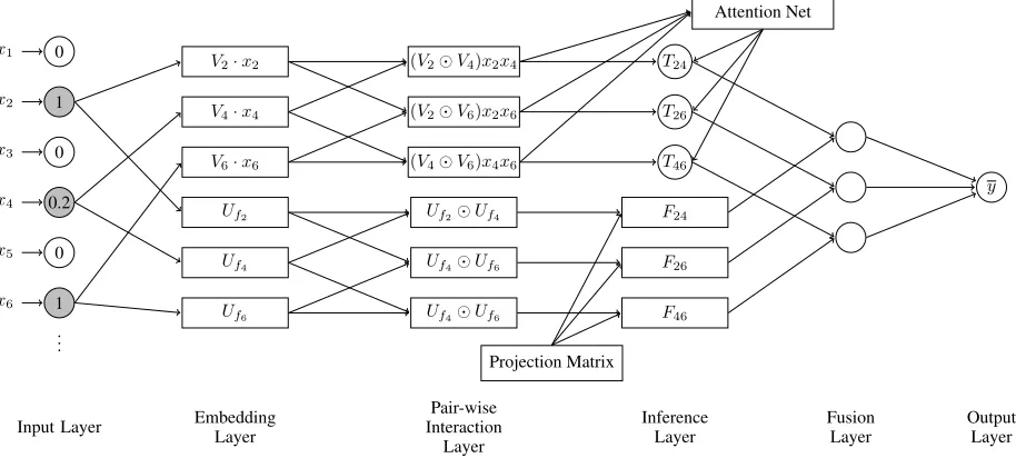
0 x1
1 x2
0 x3
0.2 x4
0 x5
1 x6
V2·x2
V4·x4
V6·x6
.. .
(V2V4)x2x4
(V2V6)x2x6
(V4V6)x4x6
Attention Net
T24
T26
T46
Uf2
Uf4
Uf6
Uf2Uf4
Uf4Uf6
Uf4Uf6
Projection Matrix F24
F26
F46
y
Input Layer Embedding Layer
Pair-wise Interaction
Layer
Inference Layer
Fusion Layer
Output Layer
Figure 1: The neural network architecture of the proposed Interaction-aware Factorization Machine (IFM).
importance, and the feature aspect has a limited impact on
the final prediction. For low temperatures (τ→0), the
prob-ability of the interaction vector with the highest expected re-ward tends to 1 and the other interactions are ignored.
The raw presentation ofFhasn(n−1)/2×Kparameters,
wherenis the number of fields, so the space complexity of
IAM is quadratic in the field number. We further factorize
tensorF using canonical decomposition(Kolda and Bader
2009):
Ffi,fj =D
T(U
fiUfj), (6)
whereU∈RKF×nandD∈
RKF×K, andK
F is the number
of latent factors of bothU andD. Therefore, the space
com-plexity is reduced toO(nKF +KFK), which is linear in
the field number.
From another perspective, field aspect learns feature in-teraction effect as a parametric similarity of the feature
interaction vector (Vi Vj)xixj and the corresponding
field interaction prototypeUfiUfj, which has a bi-linear form(Chechik et al. 2010),
simD(c, e) =cTDe, (7)
withc=UfiUfj,e= (ViVj)xixj.
Interaction-aware Factorization Machines (IFMs)
Interaction-aware Factorization Machine (IFM) models fea-ture interaction importance more precisely by introducing IAM. For simplicity, we omit linear terms and the bias term in the remaining parts. Figure 1 shows the neural network architecture of IFM, which comprises 6 layers. In the fol-lowing, several layers are detailed:• Embedding layer.The embedding layer is a fully con-nected layer that projects each feature to a dense vector
representation. IFM employs two embedding matricesV
andU for feature embedding and field embedding
query-ing, respectively.
• Pair-wise interaction layer. The pair-wise interaction layer enumerates interacted latent vectors, each of which is a element-wise product of two embedding vectors from the embedding layer. Let the feature aspect pair-wise
in-teraction setPF and the field aspect pair-wise interaction
setPI be
PF ={(ViVj)xixj |(i, j)∈X },
PI ={UfiUfj |(i, j)∈X },
(8)
then each has no information overlap; the former only
de-pends on the feature embedding matrixV, while the latter
only comes from the field embedding matrixU.
• Inference layer.The inference layer calculates thefeature aspectimportance and thefield aspectimportance accord-ing to Equation 5 and Equation 6, respectively.
To summarize, we give the overall formulation of IFM as:
y=
m
X
i=1
m
X
j=i+1
Tij(UfiUfj)
T
D(ViVj)xixj
+
m
X
i=1
wixi+w0.
(9)
We also applyL2 regularization onU andDwithλF
con-troling the regularization strength and employ dropout(Sri-vastava et al. 2014) on the pair-wise interaction layer to
prevent overfitting. Note that U∈RKF×n and V∈
RK×m
can have different dimensions; each latent vector ofU only
needs to learn the effect with a specific field, so usually,
KF K. (10)
Complexity Analysis. Feature embedding matrixV
re-quirem×Kparameters and field-aware factor importance
matrixF requiresn×KF+KF×Kparameters after
ap-plying Equation 6. Besides, the parameters of attention
isO(nKF+ (KF+m+Ka)K+ 2Ka), whereKF, Ka, K
andnare small compared tom, so the space complexity is
similar to that of FM, which isO(mK).
The cost of computingPF (Equation 8) and feature
as-pect importance are O(|X |K) and O(|X |KKa),
respec-tively. For prediction, because the field-aware factor
impor-tance matrixFcan be pre-calculated by Equation 6 and the
fusion layer only involves the inner product of two vectors,
for which the complexity isO(|X |K), the overall time
com-plexity isO(|X |KKa).
Sampling.We dynamically samplecfeature interactions according to the norms of field-aware factor importance vec-tors (Ffi,fj) and attention scores are only computed for the
sampled interactions. The cost of sampling isO(n2KFK)
for a mini-batch data and the computation cost of
atten-tion scores isO(cKKa) for every instance. By sampling,
the selection frequency for useless interactions is reduced
and the overall time complexity is reduced toO(cKKa+
n2
batchSizeKFK).
Generalized Interaction-aware Model (GIM)
We present a more generalized architecture named General-ized Interaction-aware Model (GIM) in this section and de-rive its neural network versions to effectively learn higherorder interactions. Letfeature aspectembedding setFXand
field aspectembedding setIX be
FX ={TijViVjxixj|(i, j)∈X },
IX ={DT(UfiUfj)|(i, j)∈X },
(11)
Then, the final prediction can be calculated by introducing
functionGas
y=G(FX,IX). (12) LetFXi,jandIXi,jbe the element with index(i, j)inFX
andIX, respectively. Then IFM can be seen as a special case
of GIM using the following,
GIF M(FX,IX) = X
{IXTi,jFXi,j|(i, j)∈X }. (13)
Besides, G can be a more complex function to capture
the non-linear and complex inherent structure of real-world data. Let
h0=concate{IXi,j FXi,j|(i, j)∈X },
hl=fl(Qlhl−1+zl),
(14)
wherenl is the number of nodes in the l-th hidden layer;
then,Ql∈Rnl×nl−1,z
l∈Rnlare parameters for thel-th
hid-den layer, fl is the activation function for thel-th hidden
layer, andhl∈Rnlis the output of thel-th hidden layer. Spe-cially, Interaction-aware Neural Network (INN) is defined as
GIN N(FX,IX) =hL, (15)
where L denotes the number of hidden layers and fL is
the identity function. For hidden layers, we useReluas the
activation function, which empirically shows good perfor-mance.
To learn both high- and low-order feature interactions, the wide component of DeepFM(Guo et al. 2017) is replaced by
GIF M(FX,IX)and named as DeepIFM.
Table 1: Dataset Description.
DATA SET MOVIELENS FRAPPE ORIGIN RECORDS 668,953 96,203
FEATURES 90,445 5,382
EXPERIMENTAL RECORDS 2,006,859 288,609
FIELDS 3 10
SPARSITY LEVEL 0.01% 0.19%
Experimental results
In this section, we evaluate the performance of the proposed IFM, INN and DeepIFM on two real-world datasets and ex-amine the effect of different parts of IFM. We conduct exper-iments with the aim of answering the following questions:
• RQ1 How do IFM and INN perform compared to the
state-of-the-art methods?
• RQ2How do thefeature aspectand thefield aspect(with
sampling) impact the prediction accuracy?
• RQ3How dose factorization of field-aware factor
impor-tance matrixF impact the performance of IFM?
• RQ4How do the hyparameters of IFM impact its
per-formance?
Experiment Settings
Datasets and Evaluation.We evaluate our models on two
real-world datasets, MovieLens3(Harper and Konstan 2015)
and Frappe(Baltrunas et al. 2015), for personalized tag rec-ommendation and context-aware recrec-ommendation. We fol-low the experimental settings in the previous works(Xiao et al. 2017; He and Chua 2017) and use the optimal parame-ter settings reported by the authors to have fair comparisons. The datasets are divided into a training set (70%), a probe set (20%), and a test set (10%). All models are trained on the training set, and the optimal parameters are obtained on the held-out probe set. The performance is evaluated by the
root mean square error(RMSE), where a lower score indi-cates better performance, on the test set with the optimal pa-rameters. Both datasets contain only positive records, so we generate negative samples by randomly pairing two negative samples with each log and converting each log into a feature vector via one-hot encoding. Table 1 shows a description of the datasets after processing, where the sparsity level is the ratio of observed to total features(Lee, Sun, and Lebanon 2012).
Baselines. We compare our models with the following methods:
• FM(Rendle 2010). As described in Equation 2. In
addi-tion, dropout is employed on the feature interactions to further improve its performance.
• FFM(Juan et al. 2016). Each feature has separate latent
vectors to interact with features from different fields.
3
• AFM(Xiao et al. 2017). AFM learns one coefficient for every feature interaction to enable feature interactions that contribute differently to the prediction.
• Neural Factorization Machines (NFMs)(He and Chua
2017). NFM performs a non-linear transformation on the latent space of the second-order feature interactions. Batch normalization(Ioffe and Szegedy 2015) is also em-ployed to address the covariance shift issue.
• DeepFM(Guo et al. 2017). DeepFM shares the feature
embedding between the FM and the deep component.
Regularization.We use L2 regularization, dropout, and
early stopping.
Hyperparameters.The model-independent hyperparam-eters are set to the optimal values reported by the previous works(Xiao et al. 2017; He and Chua 2017). The embedding size of features is set to 256, and the batch size is set to 4096 and 128 for MovieLens and Frappe, respectively. We also ptrain the feature embeddings with FM to get better
re-sults. For IFM and INN, we setτ = 10and tune the other
hyperparameters on the probe set.
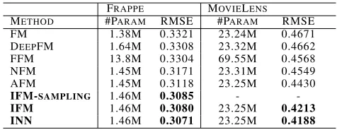
Model Performance (RQ1)
The performance of different models on the MovieLens dataset and the Frappe dataset is shown in Table 2, from which the following observations may be made:
• Learning the importance of different feature interactions
improves performance. This observation is derived from the fact that both AFM and the IAM-based models (IFM and INN) perform better than FM does. As the best model, INN outperforms FM by more than 10% and 7% on the MovieLens and Frappe datasets, respectively.
• IFM makes use of field information and can model
fea-ture interactions more precisely. To verify the effective-ness of field information, we conduct experiments with FFM and FFM-style AFM, where each feature has sepa-rate latent vectors to interact with features from different fields, on the MovieLens dataset. As expected, the utiliza-tion of field informautiliza-tion brings improvements of approx-imately 2% and 3% with respect to FM and AFM.
• INN outperforms IFM by using a more complex function
G, as described in Equation 15, which captures more com-plex and non-linear relations from IAM encoded vectors.
• Overall, our proposed IFM model outperforms the
com-petitors by more than 4.8% and 1.2% on the Movie-Lens and Frappe datasets, respectively. The proposed INN model performs even better, which achieves an improve-ment of approximately 6% and 1.5% on the MovieLens and Frappe datasets, respectively.
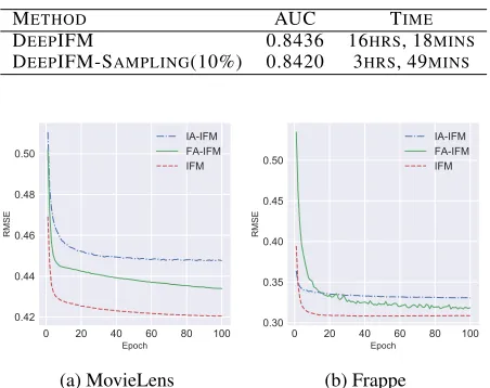
Impact of different aspects and sampling (RQ2)
IFM discriminates feature interaction importance onfeature
aspectandfield aspect. To study how each aspect influences IFM prediction, we keep only one aspect and monitor how IFM performs. As shown in Figure 2, feature-aspect-only IFM (FA-IFM) performs better than field-aspect-only IFM (IA-IFM) does. We explain this phenomenon by examining
Table 2: Test RMSE from different models.
FRAPPE MOVIELENS
METHOD #PARAM RMSE #PARAM RMSE
FM 1.38M 0.3321 23.24M 0.4671 DEEPFM 1.64M 0.3308 23.32M 0.4662 FFM 13.8M 0.3304 69.55M 0.4568 NFM 1.45M 0.3171 23.31M 0.4549 AFM 1.45M 0.3118 23.25M 0.4430
IFM-SAMPLING 1.46M 0.3085 -
-IFM 1.46M 0.3080 23.25M 0.4213 INN 1.46M 0.3071 23.25M 0.4188
the models. The FA-IFM modeling of feature interaction im-portance is more detailed for each individual interacted vec-tors; thus, it can make use of the feature interaction infor-mation precisely, whereas IA-IFM utilizes only field-level interaction information and lacks the capacity to distinguish feature interactions from the same fields. Although FA-IFM models feature interactions in a more precise way, IFM still achieves a significant improvement by incorporating field in-formation, which can be seen as auxiliary inin-formation, to give more structured control and allow for more leverage when tweaking the interaction between features.
We now focus on analyzing the different role of field as-pect in different datasets. We calculated the ratio of the im-provements of FA-IFM over IA-IFM, which were 9:1 and 1.7:1 on the Frappe and MovieLens datasets, respectively. It is determined that field information plays a more significant role in the MovieLens dataset. We explain this phenomenon by examining the datasets. As shown in Table 1, the Movie-Lens dataset is sparser than the Frappe dataset, where the field information brings more benefit(Juan et al. 2016).
Field importance Analysis. Field aspect not only im-proves the model performance but also gives the ability to interpret the importance of feature interactions at the field-factor level. Besides, the norm of field aspect importance vector provides insight into interaction importance at the field level. To demonstrate this, we investigate field aspect importance vectors on the MovieLens dataset. As shown in Table 3, the movie-tag interaction is the most impor-tant while the user-movie interaction has a negligible im-pact on the prediction because tags link users and items as a bridge(Chen et al. 2016) and directly modeling semantic correlation between them is less effective.
Sampling.To examine how sampling affects the perfor-mance of IFM, an experiment was conducted on Frappe dataset and because there are only three interactions in MovieLens dataset, sampling is meaningless. As shown in Table 2, IFM with sampling achieves a similar level of performance. To verify how sampling performs when the
dataset is large, we compare the performance4 on
click-through prediction for advertising in Tencent video, which
has around 10 billion instances. As shown in Table 4, sam-pling reduce the training time with no significant loss to the performance.
4
Table 3: The norm of field aspect importance vector of each feature interaction on the MovieLens dataset.
USER-MOVIE USER-TAG MOVIE-TAG
NORM 0.648 5.938 9.985
PROPORTION 3.9 % 35.8 % 60.3 %
Table 4: The performance on click-through prediction for advertising inTencent video.
METHOD AUC TIME
DEEPIFM 0.8436 16HRS, 18MINS DEEPIFM-SAMPLING(10%) 0.8420 3HRS, 49MINS
0 20 40 60 80 100
Epoch
0.42 0.44 0.46 0.48 0.50
RMSE
IA-IFM FA-IFM IFM
(a) MovieLens
0 20 40 60 80 100
Epoch
0.30 0.35 0.40 0.45 0.50
RMSE
IA-IFM FA-IFM IFM
(b) Frappe
Figure 2: Comparison of test RMSE by using only one as-pect.
Impact of factorization (RQ3)
As described in Equation 6, IAM factorizes field-aware fac-tor importance matrixF∈Rn(n−1)/2×K to get a more com-pact representation. We conduct experiments with both the factorized version and the non-factorized version (indicated
as IFM−) to determine how factorization affects the
perfor-mance. As shown in Figure 3, factorization can speed up the convergence of both datasets. However, it also has a sig-nificantly different impact on the performance of the two datasets. For the MovieLens dataset, both versions achieve
similar levels of performance but IFM outperforms IFM−by
a large margin on the Frappe dataset, where the performance
of IFM− is degraded from epoch 50 because of an
overfit-ting issue5. We explain this phenomenon by comparing the
number of entries of field-aware factor importance matrix
F. For the Frappe dataset, IFM− and IFM have 11,520 and
6,370 entries with the optimal settings withK = 256and
KF = 26, respectively. That is, after factorization, we can
reduce more than 44% of the parameters, thereby signifi-cantly reducing the model complexity. In contrast to that, the MovieLens dataset contains only three interactions, where
the effect of factorization is negligible and IFM− performs
slightly better than IFM does although the gap is negligible, i.e., around 0.1%.
5
Early stopping is disabled in this experiment.
0 20 40 60 80 100
Epoch
0.43 0.44 0.45 0.46 0.47 0.48
RMSE
IFM
IFM
(a) MovieLens
0 25 50 75 100
Epoch
0.300 0.325 0.350 0.375 0.400 0.425 0.450 0.475
RMSE
IFM
IFM
(b) Frappe
Figure 3: Performance comparison on the test setw.r.t.IFM
and the non-factorization version IFM-.
0.2 0.4 0.6 0.8 1.0
keep prob
0.42 0.43 0.44 0.45 0.46 0.47 0.48 0.49 0.50
RMSE
IFM FM
(a) MovieLens
0.2 0.4 0.6 0.8 1.0
keep prob
0.31 0.32 0.33 0.34 0.35 0.36 0.37 0.38
RMSE
IFM FM
(b) Frappe
Figure 4: Comparison of test RMSE by varying keep proba-bilities.
0 0.001 0.01 0.1 1
F
0.421 0.422 0.423 0.424 0.425 0.426 0.427
RMSE
(a) MovieLens
0 0.001 0.01 0.1
F
0.32 0.34 0.36 0.38 0.40
RMSE
(b) Frappe
Figure 5: Comparison of test RMSE by varyingλF.
Effect of Hyper-parameters (RQ4)
4 8 16 32 64 128 KF
0.422 0.423 0.424 0.425
RMSE
(a) MovieLens
8 16 26 32 64 128 KF
0.308 0.309 0.310 0.311 0.312
RMSE
(b) Frappe
Figure 6: Comparison of test RMSE by varyingKF.
probability tends to 1, i.e., no dropout is employed, both models also cannot achieve the best performance. Both IFM and FM achieve the best performance when the keep proba-bility is properly set due to the extreme bagging effect. For nearly all keep probabilities, IFM outperforms FM, which shows the effectiveness of IAM.
L2 regularization. Figure 5 shows how IFM performs
when theL2regularization hyperparameterλFvaries while
keeping the dropout ratio constant (optimal value from the
validation dataset). IFM performs better when L2
regular-ization is applied and it achieves an improvement of approx-imately 1.4% in the MovieLens dataset. We explain this phe-nomenon as the following. Using dropout on the pair-wise interaction layer only prevent overfitting for the feature
as-pect andλFcontrols the regularization strength of
factoriza-tion parameters for the field aspect importance learning.
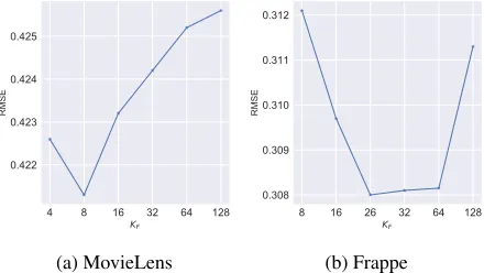
The number of hidden factorsKF.Figure 6 shows how
IFM performs when the number of hidden factorsKFvaries.
IFM cannot effectively capture the field-aware factor
im-portance whenKF is small and it also can not achieve the
best performance whenKF is large due to the overfitting
is-sue. An interesting phenomenon is that the bestKF for the
MovieLens dataset is much smaller than that for the Frappe dataset. We explain this phenomenon by looking into the
datasets. Because the number of fieldsnis 10 for the Frappe
dataset, the field-aware factor importance matrix captures the importance of factors from 45 interacted vectors. While the MovieLens dataset contains only 3 interactions and the field-aware factor importance matrix keeps much less infor-mation.
Related work
In the introduction section, factorization machine and its many neural network variants are already mentioned, thus we do not discuss them here. In what follows, we briefly re-capitulate the two most related models, i.e., AFM(Xiao et al. 2017) and FFM(Juan et al. 2016).
AFM learns one coefficient for every feature interaction to enable feature interactions that contribute differently to the final prediction and the importance of a feature interaction is automatically learned from data without any human domain knowledge. However, the pooling layer of AFM lacks the ca-pacity of discriminating factor importance in feature
interac-tions from different fields. In contrast, IFM models feature interaction importance at interaction-factor level; thus, the same factor in different interactions can have significantly different influences on the final prediction.
In FMs, every feature has only one latent vector to learn the latent effect with any other features. FFM utilizes field information as auxiliary information to improve model per-formance and introduces more structured control. In FFM, each feature has separate latent vectors to interact with fea-tures from different fields, thus the effect of a feature can differ when interacting with features from different fields. However, modeling feature interactions without discriminat-ing importance is unreasonable. IFM learns flexible inter-action importance and outperforms FFM by more than 6% and 7% on the Frappe and MovieLens datasets, respectively.
Moreover, FFM requires O(mnK) parameters, while the
space complexity of IFM isO(mK).
Conclusion and Future Directions
In this paper, we proposed a generalized interaction-aware model and its specialized versions to improve the represen-tation ability of FM. They gain performance improvement based on the following advantages. (1) All models can ef-fectively learn both the feature aspect and the field aspect interaction importance. (2) All models can utilize field in-formation that is usually ignored but useful. (3) All models apply factorization in a stratified manner. (4) INN and Deep-IFM can learn jointly with deep representations to capture the non-linear and complex inherent structure of real-world data.
The experimental results on two well-known datasets show the superiority of the proposed models over the state-of-the-art methods. To the best of our knowledge, this work represents the first step towards absorbing field information into feature interaction importance learning.
In the future, we would like to generalize the field-aware importance matrix to a more flexible structure by applying neural architecture search(Liu et al. 2017).
References
Baltrunas, L.; Church, K.; Karatzoglou, A.; and Oliver, N. 2015. Frappe: Understanding the usage and perception of
mobile app recommendations in-the-wild. arXiv preprint
arXiv:1505.03014.
Cao, B.; Zhou, H.; Li, G.; and Yu, P. S. 2016.
Multi-view machines. InProceedings of the Ninth ACM
Interna-tional Conference on Web Search and Data Mining, 427– 436. ACM.
Chang, Y.-W.; Hsieh, C.-J.; Chang, K.-W.; Ringgaard, M.; and Lin, C.-J. 2010. Training and testing low-degree
poly-nomial data mappings via linear svm. Journal of Machine
Learning Research11(Apr):1471–1490.
Chechik, G.; Sharma, V.; Shalit, U.; and Bengio, S.
2010. Large scale online learning of image similarity
through ranking. Journal of Machine Learning Research
Chen, C.; Zheng, X.; Wang, Y.; Hong, F.; Lin, Z.; et al. 2014. Context-aware collaborative topic regression with social
ma-trix factorization for recommender systems. InAAAI, 9–15.
Chen, C.; Zheng, X.; Wang, Y.; Hong, F.; Chen, D.; et al. 2016. Capturing semantic correlation for item
recommen-dation in tagging systems. InAAAI, 108–114.
Chen, J.; Zhang, H.; He, X.; Nie, L.; Liu, W.; and Chua, T.-S. 2017. Attentive collaborative filtering: Multimedia recommendation with item-and component-level attention. In Proceedings of the 40th International ACM SIGIR con-ference on Research and Development in Information Re-trieval, 335–344. ACM.
Cheng, H.-T.; Koc, L.; Harmsen, J.; Shaked, T.; Chandra, T.; Aradhye, H.; Anderson, G.; Corrado, G.; Chai, W.; Ispir, M.; et al. 2016. Wide & deep learning for recommender systems. In Proceedings of the 1st Workshop on Deep Learning for Recommender Systems, 7–10. ACM.
Guo, H.; Tang, R.; Ye, Y.; Li, Z.; and He, X. 2017. Deepfm: a factorization-machine based neural network for ctr
predic-tion. InProceedings of the 26th International Joint
Confer-ence on Artificial IntelligConfer-ence, 1725–1731. AAAI Press. Harper, F. M., and Konstan, J. A. 2015. The movielens
datasets: History and context. ACM Transactions on
Inter-active Intelligent Systems (TiiS)5(4):19.
He, X., and Chua, T.-S. 2017. Neural factorization
ma-chines for sparse predictive analytics. InProceedings of the
40th International ACM SIGIR conference on Research and Development in Information Retrieval, 355–364. ACM.
Hinton, G.; Vinyals, O.; and Dean, J. 2015.
Distill-ing the knowledge in a neural network. arXiv preprint
arXiv:1503.02531.
Hong, F.-X.; Zheng, X.-L.; and Chen, C.-C. 2016. Latent
space regularization for recommender systems.Information
Sciences360:202–216.
Ioffe, S., and Szegedy, C. 2015. Batch normalization: Accel-erating deep network training by reducing internal covariate
shift. In International Conference on Machine Learning,
448–456.
Juan, Y.; Zhuang, Y.; Chin, W.-S.; and Lin, C.-J. 2016.
Field-aware factorization machines for ctr prediction. In
Proceed-ings of the 10th ACM Conference on Recommender Systems, 43–50. ACM.
Kolda, T. G., and Bader, B. W. 2009. Tensor decompositions
and applications. SIAM review51(3):455–500.
Koren, Y. 2008. Factorization meets the neighborhood: a
multifaceted collaborative filtering model. InProceedings of
the 14th ACM SIGKDD international conference on Knowl-edge discovery and data mining, 426–434. ACM.
Lee, J.; Sun, M.; and Lebanon, G. 2012. A comparative
study of collaborative filtering algorithms. arXiv preprint
arXiv:1205.3193.
Liu, C.; Zoph, B.; Shlens, J.; Hua, W.; Li, L.-J.;
Fei-Fei, L.; Yuille, A.; Huang, J.; and Murphy, K. 2017.
Progressive neural architecture search. arXiv preprint
arXiv:1712.00559.
McMahan, H. B.; Holt, G.; Sculley, D.; Young, M.; Ebner, D.; Grady, J.; Nie, L.; Phillips, T.; Davydov, E.; Golovin, D.; et al. 2013. Ad click prediction: a view from the trenches. In
Proceedings of the 19th ACM SIGKDD international confer-ence on Knowledge discovery and data mining, 1222–1230. ACM.
Qu, Y.; Cai, H.; Ren, K.; Zhang, W.; Yu, Y.; Wen, Y.; and Wang, J. 2016. Product-based neural networks for user
re-sponse prediction. InData Mining (ICDM), 2016 IEEE 16th
International Conference on, 1149–1154. IEEE.
Rendle, S., and Schmidt-Thieme, L. 2010. Pairwise interac-tion tensor factorizainterac-tion for personalized tag
recommenda-tion. InProceedings of the third ACM international
confer-ence on Web search and data mining, 81–90. ACM.
Rendle, S. 2010. Factorization machines. InData Mining
(ICDM), 2010 IEEE 10th International Conference on, 995– 1000. IEEE.
Srivastava, N.; Hinton, G.; Krizhevsky, A.; Sutskever, I.; and Salakhutdinov, R. 2014. Dropout: A simple way to prevent
neural networks from overfitting. The Journal of Machine
Learning Research15(1):1929–1958.
Wang, P.; Guo, J.; Lan, Y.; Xu, J.; Wan, S.; and Cheng, X. 2015. Learning hierarchical representation model for
nextbasket recommendation. InProceedings of the 38th
In-ternational ACM SIGIR conference on Research and Devel-opment in Information Retrieval, 403–412. ACM.
Wang, R.; Fu, B.; Fu, G.; and Wang, M. 2017. Deep &
cross network for ad click predictions. InProceedings of the
ADKDD’17, 12. ACM.
Xiao, J.; Ye, H.; He, X.; Zhang, H.; Wu, F.; and Chua, T.-S. 2017. Attentional factorization machines: Learning the
weight of feature interactions via attention networks. In
Pro-ceedings of the Twenty-Sixth International Joint Conference on Artificial Intelligence (IJCAI-17). Morgan Kaufmann. Zhang, W.; Du, T.; and Wang, J. 2016. Deep learning over
multi-field categorical data. InEuropean conference on