Time for a Change: a Tutorial for Comparing Multiple
Classifiers Through Bayesian Analysis
Alessio Benavoli† [email protected]
Giorgio Corani† [email protected]
Janez Demˇsar\
Marco Zaffalon† [email protected]
\Faculty of Computer and Information Science, University of Ljubljana,
Vecna pot 113, SI-1000 Ljubljana, Slovenia
†Istituto Dalle Molle di Studi sull’Intelligenza Artificiale (IDSIA)
Galleria 2, 6928 Manno, Switzerland
Editor:David Barber
Abstract
The machine learning community adopted the use of null hypothesis significance testing (NHST) in order to ensure the statistical validity of results. Many scientific fields however realized the shortcomings of frequentist reasoning and in the most radical cases even banned its use in publications. We should do the same: just as we have embraced the Bayesian paradigm in the development of new machine learning methods, so we should also use it in the analysis of our own results. We argue for abandonment of NHST by exposing its fallacies and, more importantly, offer better—more sound and useful—alternatives for it.
Keywords: comparing classifiers, null hypothesis significance testing, pitfalls of p-values, Bayesian hypothesis tests, Bayesian correlated test, Bayesian hierarchical correlated t-test, Bayesian signed-rank test
1. Introduction
Progression of Science and of the scientific method go hand in hand. Development of new theories requires—and at the same time facilitates—development of new methods for their validation.
Pioneers of machine learning were playing with ideas: new approaches, such as induc-tion of classificainduc-tion trees, were worthy of publicainduc-tion for the sake of their interestingness. As the field progressed and found more practical uses, variations of similar ideas began emerging, and with that the interest in determining which of them work better in prac-tice. A typical example are the different measures for assessing the quality of attributes; deciding which work better than others required tests on actual, real-world data. Papers thus kept introducing new methods and measured, for instance, classification accuracies to prove their advantages over the existing methods. To ensure the validity of such claims, we adopted—starting with the work of Dietterich (1998) and Salzberg (1997), and later followed by Demˇsar (2006)—the common statistical methodology used in all scientific areas relying on empirical observations: the null hypothesis significance testing (NHST).
c
This spread the understanding that the observed results require statistical validation. On the other hand, NHST soon proved inadequate for many reasons (Demˇsar, 2008). Note-worthy, the American Statistical Association has recently made a statement against p-values (Wasserstein and Lazar, 2016). NHST nowadays it is also falling out of favour in other fields of science (Trafimow and Marks, 2015). We believe that the field of machine learning is ripe for a change as well.
We will spend a whole section demonstrating the many problems of NHST. In a nutshell: it does not answer the question we ask. In a typical scenario, a researcher proposes a new method and desires to prove that it is more accurate than another method on a single data set or on a collection of data sets. She thus runs the competing methods and records their results (classification accuracy or another appropriate score) on one or more data sets, which is followed by NHST. The difference between what the researcher has in mind and what the NHST provides for is evident from the following quote from a recently published paper: “Therefore, at the 90% confidence level, we can conclude that (...) method is able to significantly outperform the other approaches.” This is wrong. The stated 90% confidence level is not the probability of one classifier outperforming another. The NHST computes the probability of getting the observed (or a larger) difference between classifiers if the null hypothesis of equivalence was true, which is not the probability of one classifier being more accurate than another, given the observed empirical results. Another common problem is that the claimed statistical significance might have no practical impact. Indeed, the common usage of NHST relies on the wrong assumptions that the p-value is a reasonable proxy for the probability of the null hypothesis and that statistical significance implies practical significance.
As we wrote at the beginning, development of Science not only requires but also facili-tates the improvement of scientific methods. Advancement of computational techniques and power reinvigorated the interest for Bayesian statistics. Bayesian modelling is now widely adopted for designing principled algorithms for learning from data (Bishop, 2007; Murphy, 2012). It is time to also switch to Bayesian statistics when it comes to analysis of our own results.
The questions we are actually interested in—e.g., is method A better than B? Based on the experiments, how probably is A better? How high is the probability that A is better by more than 1%?—are questions about posterior probabilities. These are naturally provided by the Bayesian methods (Edwards et al., 1963; Dickey, 1973; Berger and Sellke, 1987). The core of this paper is thus a section that establishes the Bayesian alternatives to frequentist NHST and discusses their inference and results. We eventually describe also the software libraries with the necessary algorithms and give short instructions for their use.
2. Frequentist analysis of experimental results
1. choose a comparison metric;
2. select a group of datasets to evaluate the algorithms;
3. perform m runs ofk-fold cross-validation for each classifier on each dataset.
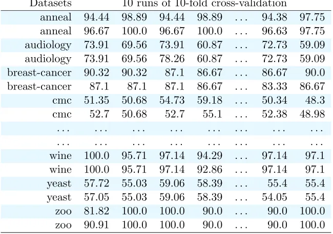
We have performed these steps in WEKA, choosing accuracy as metric, on a collection of 54 data sets downloaded from the the WEKA website1 and with 10 runs of 10-fold cross-validation. Table 1 reports the accuracies obtained on each dataset by each classifier. First of all, we aim at knowing which is the best classifier for each dataset. The an-swer to this question is probabilistic, since on each data set we have only estimates of the performance of each classifier.
Datasets 10 runs of 10-fold cross-validation
anneal 94.44 98.89 94.44 98.89 . . . 94.38 97.75 anneal 96.67 100.0 96.67 100.0 . . . 96.63 97.75 audiology 73.91 69.56 73.91 60.87 . . . 72.73 59.09 audiology 73.91 69.56 78.26 60.87 . . . 72.73 59.09 breast-cancer 90.32 90.32 87.1 86.67 . . . 86.67 90.0 breast-cancer 87.1 87.1 87.1 86.67 . . . 83.33 86.67 cmc 51.35 50.68 54.73 59.18 . . . 50.34 48.3 cmc 52.7 50.68 52.7 55.1 . . . 52.38 48.98 . . . . . . . . wine 100.0 95.71 97.14 94.29 . . . 97.14 97.1 wine 100.0 95.71 97.14 92.86 . . . 97.14 97.1 yeast 57.72 55.03 59.06 58.39 . . . 55.4 55.4 yeast 57.05 55.03 59.06 58.39 . . . 54.05 55.4 zoo 81.82 100.0 100.0 90.0 . . . 90.0 100.0 zoo 90.91 100.0 100.0 90.0 . . . 90.0 100.0
Table 1: Accuracies for 10 runs of 10-fold cross-validation on 54 UCI datasets fornbc (blue row) versusaode (white rows).
.
Since during cross-validation we have provided both classifiers with the same training and test sets, we can compare the classifiers by considering the difference in accuracies on each test set. This yields the vector of differences of accuracies x = {x1, x2, . . . , xn}, where n = 100 (10 runs of 10-fold cross-validation). We can compute the mean of the vector of differencesx, i.e., the mean difference of accuracy between the two classifiers, and statistically evaluate whether the mean difference is significantly different from zero. In frequentist analysis, we would perform a NHST using the t-test. The problem is that the
t-test assumes the observations to be independent. However, the differences of accuracies
are not independent of each other because of the overlapping training sets used in cross-validation. Thus the usual t-test is not calibrated when applied to the analysis of cross-validation results: when sampling the data under the null hypothesis its rate of Type I errors is much larger than α (Dietterich, 1998). Moreover, the correlation cannot be estimated from data; Nadeau and Bengio (2003) have proven that there is no unbiased estimator of the correlation of the results obtained on the different folds. Introducing some approximations, they have proposed a heuristic to choose the correlation parameter: ρ = ntotnte, where nte,
ntr and ntot =nte+ntr respectively denote the size of the training set, of the test set and of the whole available data set.2
Frequentist correlated t-test
The correlatedt-test is based on the modified Student’s t-statistic:
t(x, µ) = q x−µ
ˆ
σ2(1 n+
ρ 1−ρ)
= q x−µ
ˆ
σ2(1 n +
nte ntr)
, (1)
where x = 1nPn
i=1xi and ˆσ =
q
1 n−1
Pn
i=1(xi−x)2 are the sample mean and sample standard deviation of the datax,ρis the correlation between the observations andµis the value of the mean we aim at testing. The statistic follows a Student distribution withn−1 degrees of freedom:
St
¯
x;n−1, µ,
1
n+
ρ
1−ρ
ˆ
σ2
. (2)
For ρ = 0, we obtain the traditional t-test. For ρ = ntotnte, we obtain the correlated t -test proposed by Nadeau and Bengio (2003) to account for the correlation due to the overlapping training sets. Usually the test is run in a two-sided fashion. Its hypotheses are:
H0:µ= 0; H1:µ6= 0. The p-value of the statistic under the null hypotheses is:
p= 2·(1− Tn−1(|t(x,0)|)), (3)
whereTn−1(|t(x,0)|) denotes the cumulative distribution of the standardized Student distri-bution withn−1 degrees of freedom in|t(x, µ)|forµ= 0. For instance, for the first data set in Table 1 we have that ¯x=−0.0194, ˆσ = 0.01583,ρ= 1/10,n= 100 and sot(¯x,0) =−3.52. Hence, the two-sidedp-value isp = 2·(1− Tn−1(|t(x,0)|)) = 0.00065≈0.001. Sometimes the directional one-sided test is performed. If the alternative hypothesis is the positive one, the hypotheses of the one-sided test are: H0 : µ ≤ 0; H1 : µ > 0. The p-value is
p= 1− Tn−1(t(x,0)).
Table 2 reports the two-sidedp-values for each comparison on each dataset obtained via the correlated t-test. The common practice in NHST is to declare all the comparisons such that p≤0.05 as significant, i.e., the accuracy of the two classifiers is significantly different on that dataset. Conversely, all the comparisons withp >0.05 are declared not significant.
Note that these significance tests can, under the NHST paradigm, only be considered in isolation, while combined they require either an omnibus test like ANOVA or corrections for multiple comparisons.
Dataset p-value Dataset p-value Dataset p-value
anneal 0.001 audiology 0.622 breast-cancer 0.598
cmc 0.338 contact-lenses 0.643 credit 0.479
german-credit 0.171 pima-diabetes 0.781 ecoli 0.001
eucalyptus 0.258 glass 0.162 grub-damage 0.090
haberman 0.671 hayes-roth 1.000 cleeland-14 0.525
hungarian-14 0.878 hepatitis 0.048 hypothyroid 0.287
ionosphere 0.684 iris 0.000 kr-s-kp 0.646
labor 1.000 lier-disorders 0.270 lymphography 0.018
monks1 0.000 monks3 0.220 monks 0.000
mushroom 0.000 nursery 0.000 optdigits 0.000
page 0.687 pasture 0.000 pendigits 0.452
postoperatie 0.582 primary-tumor 0.492 segment 0.000 solar-flare-C 0.035 solar-flare-m 0.596 solar-flare-X 0.004
sonar 0.777 soybean 0.049 spambase 0.000
spect-reordered 0.198 splice 0.004 squash-stored 0.940
squash-unstored 0.304 tae 0.684 credit 0.000
owel 0.000 waveform 0.417 white-clover 0.463
wine 0.671 yeast 0.576 zoo 0.435
Table 2: Two sided p-values for each dataset. The difference is significant (p <0.05) in 19 out of 54 comparisons.
2.1 NHST: the pitfalls of black and white thinking
Despite being criticized from its inception, NHST is still considered necessary for publica-tion, as p ≤0.05 is trusted as an objective proof of the method’s quality. One of the key problems of decisions based on p ≤ 0.05 is that it leads to “black and white thinking”, which ignores the fact that (i) a statistically significant difference is completely different from a practically significant difference (Berger and Sellke, 1987); (ii) two methods that are not statistically significantly different are not necessarily equivalent. The NHST and thisp-value-related “black and white thinking” do not allow for making informed decisions. Hereafter, we list the limits of NHST in order of severity using, as a working example, the assessment of the performance of classifiers.
NHST does not estimate probabilities of hypotheses. What is the probability that the performance of two classifiers is different (or equal)? This isthe question we are asking when we compare two classifiers; and NHST cannot answer it.
τ|H0), wheret(x) is the statistic computed from the datax, andτ is the critical value cor-responding to the test and the selected α. This is not the probability of the hypothesis,
p(H0|x), in which we are interested.
Yet, researchers want to know the probability of the null and the alternative hypotheses on the basis of the observed data, rather than the probability of the data assuming the null hypothesis to be true. Sentences like “at the 95% confidence level, we can conclude that(...)”, are formally correct, but they seem to imply that 1−p is the probability of the alternative hypothesis, while in fact 1−p= 1−p(t(x)> τ|H0) =p(t(x)< τ|H0), which is not the same asp(H1|x). This is summed up in Table 3.
what we compute what we would like to know
p(t(x)> τ|H0) p(H0|x)
1−p(t(x)> τ|H0) =p(t(x)< τ|H0) 1−p(H0|x) =p(H1|x)
Table 3: Difference between the probabilities of interest for the analyst and the probabilities computed by the frequentist test.
Point-wise null hypotheses are practically always false. The difference between two classifiers can be very small; however there are no two classifiers whose accuracies are perfectly equivalent.
By using a NHST, the null hypothesis is that the classifiers are equal. However, the null hypothesis is practically always false! By rejecting the null hypothesis NHST indicates that the null hypothesis is unlikely; but this is known even before running the experiment. This problem of the NHST has been pointed out in many different scientific domains (Lecoutre and Poitevineau, 2014, Sec 4.1.2.2). A consequence is that, since the null hypothesis is always false, by adding enough data points it is possible to claim significance even when the effect size is trivial. This is because the p-value is affected both by the sample size and the effect size, as discussed in the next section. Quoting Kruschke and Liddell (2015): “null hypotheses are straw men that can virtually always be rejected with enough data.”
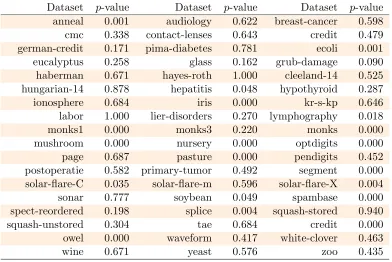
The p-value does not separate between the effect size and the sample size. The usual explanation for this phenomenon is that if the effect size H0 is small, more data is needed to demonstrate the difference. Enough data can confirm arbitrarily small effects. Since the sample size is manipulated by the researcher and the null hypothesis is always wrong,the researcher can reject it by testing the classifiers on enough data. On the contrary, conceivable differences may fail to yield smallp-values if there are not enough suitable data for testing the method (e.g., not enough datasets). Even if we pay attention not to confuse thep-value with the probability of the null hypothesis, thep-value is intuitively understood as the indicator of the effect size. In practice, it is the function of effect size and sample size: samep-values do not imply same effect sizes.
define the region in which the differences of accuracy is less than 1%—the meaning of these lines will be clarified in the next sections.
The p-value is 0.077 in the first case and so the null hypothesis cannot be rejected. The p-value becomes 0.048 in the second case and so the null hypothesis can be rejected. This demonstrates how adding data leads to rejection of the null hypothesis although the difference between the two classifiers is very small in this dataset (all the mass is inside the two orange vertical lines). Practical significance can be equated with the effect size, which is what the researcher is interested in. Statistical significance—the p-value—is not a measure of practical significance, as shown in the example.
DeltaAcc
-0.02 -0.01 0.00 0.01 0.02
0 50 100 150
DeltaAcc
-0.02 -0.01 0.00 0.01 0.02
0 50 100 150
Figure 1: Density plot for the differences of accuracy betweennbc and aode for the dataset hepatitisconsidering only 15 of the 100 data (left) or all the data (right). Left: the null hypothesis cannot be rejected (p= 0.077>0.05) using half the data. Right: the null hypothesis is rejected when all the data are considered (p= 0.048<0.05), despite the very small effect size.
DeltaAcc
-0.25 -0.20 -0.15 -0.10 -0.05 0.00 0.05 0.10 0
2 4 6 8
DeltaAcc
-0.25 -0.20 -0.15 -0.10 -0.05 0.00 0.05 0.10 0
10 20 30
Figure 2: Density plot for the differences of accuracy (DeltaAcc) betweennbc andaode for the datasetsecoli (left) andiris(right). The null hypothesis is rejected (p <0.05) with similarp-values, even though the two cases have very different uncertainty. Forecoli, the uncertainty is very large and includes zero.
NHST yields no information about the null hypothesis. What can we say when NHST does not reject the null hypothesis?
The scientific literature contains examples of non-significant tests interpreted as evidence of no difference between the two methods/groups being compared. This is wrong since NHST cannot provide evidence in favour of the null hypothesis (see also Lecoutre and Poitevineau (2014, Sec 4.1.2.2) for further examples on this point). When NHST does not reject the null hypothesis, no conclusion can be made.
Researchers may be interested in the probability that two classifiers are equivalent. For instance, a recent paper contains the following conclusion: “there is no significant difference between (...) under the significance level of 0.05. This is quite a remarkable conclusion.” This is not correct, we cannot conclude anything in this case! Consider for example Figure 3 (left), which shows the density plot of the differences of accuracy between nbc and aode for the datasetaudiology. The correlated t-test gives a p-valuep= 0.622 and so it fails to reject the null hypothesis. However, NHST does not allow us to reach any conclusion about the possibility that the two classifiers may actually be equivalent in this dataset, although the majority of data (density plot) seems to support this hypothesis. We tend to interpret these cases as acceptance of the null hypothesis or to even (mis)understand thepvalue as a “62.2% probability that the performance of the classifiers is the same”. This is also evident from Figure 3 (right), where a very similar p-value, p = 0.598, corresponds to a different density plot—with more uncertainty and so less evidence in favour of the null.
DeltaAcc
-0.10 -0.05 0.00 0.05 0.10 0
20 40 60 80
DeltaAcc
-0.10 -0.05 0.00 0.05 0.10 0
5 10 15 20 25
Figure 3: Density plot for the differences of accuracy betweennbc andaodefor the datasets audiology (left) andbreast-cancer (right). Inaudiology, we can only say that the null hypothesis cannot be rejectedp= 0.622 (>0.05). NHST does not allow the conclusion that the null hypothesis is true although practically all the data lies in the interval [−0.01,0.01] (the differences of accuracy are less than 1%). A similar
p-value corresponds to a very different situation forbreast-cancer.
We pretend thatαis the proportion of cases in whichH0 would be falsely rejected if the same experiment was repeated. This would be true if thep-value represented the probability of the null hypothesis. In reality, α is the proportion of cases in which experiments yield the data that is more extreme than expected under H0; the actual probability of falsely rejecting H0 is also related to the probability ofH0 and the data.
For α to be meaningful, it would need to set the required effect size or at least the probability of the hypothesis, not the likelihood of the data.
The inference depends on the sampling intention. Consider analysing a data set of n observations with a NHST test. The sampling distribution used to determine the critical value of the test assumes that our intention was to collect exactly nobservations. If the intention was different—for instance in machine learning you typically compare two algorithms on all the datasets that are available—, the sampling distribution changes to reflect the actual sampling intentions (Kruschke, 2010). This is never done, given the difficulty of formalizing one’s intention and of devising an appropriate sampling distribution. This problem is thus important but generally ignored. Thus for the data set the hypothesis test (and thus the p-value) should be computed differently, depending on the intention of the person who collected the data (Kruschke, 2010).
3. Bayesian analysis of experimental results
The second Bayesian approach does not set any null value. The analyst simply has to set up a range of candidate values (prior model), including the zero effect, and use Bayesian inference to compute the relative credibilities of all the candidate values (the posterior distribution). This method is called Bayesian estimation (Gelman et al., 2014; Kruschke, 2015).
The choice of the method depends on the situation – is a point-wise null hypothesis plausible ? (Bayarri and Berger, 2013, Sec.18.2.3.1)
In machine learning the estimation approach is preferable because there is not plausible reason to believe that two different classifiers have exactly the same accuracy. For this reason, we will focus on the Bayesian estimation approach that hereafter we will simply call Bayesian analysis.
The first step in Bayesian analysis is establishing a descriptive mathematical model of the data. In a parametric model, this mathematical model is the thelikelihood function that provides the probability of the observed data for each candidate value of the parameter(s)
p(Data|θ). The second step is to establish the credibility for each value of the parameter(s) before observing data, the prior distribution p(θ). The third step is to use Bayes’ rule to combine likelihood and prior to obtain the posterior distribution of the parameter(s) given the datap(θ|Data). The questions we pose in statistical analysis can be answered by querying this posterior distribution in different ways.
As a concrete example of Bayesian analysis we will compare the accuracies of two com-peting classifiers via cross-validation on multiple data sets (Table 1). For this purpose, we will adopt thecorrelated Bayesian t-test proposed by Corani and Benavoli (2015).
Bayesian correlated t-test
The Bayesian correlated t-test is used for the analysis of cross-validation results on a single dataset and it accounts for the correlation due to the overlapping training sets. The test is based on the following (generative) model of the data:
xn×1 =1n×1µ+vn×1, (4)
where x= (x1, x2, . . . , xn) is the vector of differences of accuracy,1n×1 is a vector of ones, µ is the parameter of interest (the mean difference of accuracy) andv∼MVN(0,Σn×n) is a multivariate Normal noise with zero mean and covariance matrix Σn×n. The covariance matrixΣis characterized as follows: Σii=σ2 and Σij =σ2ρfor alli6=j∈1, . . . , n, where
ρ is the correlation and σ2 is the variance and, therefore, the covariance matrix takes into account the correlation due to cross-validation. Hence, the likelihood model of data is
p(x|µ,Σ) = exp(− 1
2(x−1µ)TΣ
−1(x−1µ))
(2π)n/2p
|Σ| . (5)
The likelihood (5) does not allow to estimate ρ from data, since the maximum likelihood estimate of ρ is ˆρ = 0 regardless the observations (Corani and Benavoli, 2015). This confirms that ρ is not identifiable: thus the Bayesian correlated t-test adopts the same heuristicρ = ntotnte suggested by Nadeau and Bengio (2003).
end, we consider the following prior:
p(µ, ν|µ0, k0, a, b) =N
µ;µ0,
k0
ν
G(ν;a, b) =N G(µ, ν;µ0, k0, a, b),
which is a Normal-Gamma distribution (Bernardo and Smith, 2009, Chap. 5) with parame-ters (µ0, k0, a, b). The Normal-Gamma prior is conjugate to the likelihood (5). If we choose the prior parameters {µ0 = 0, k0 → ∞, a= −1/2, b= 0} (matching prior), the resulting posterior distribution of µis the following Student distribution:
p(µ|x, µ0, k0, a, b) =St
µ;n−1,x,¯
1
n +
ρ
1−ρ
ˆ
σ2
, (6)
where ¯x =
Pn i=1xi
n and ˆσ
2 = Pni=1(xi−x)¯ 2
n−1 . For these values of the prior parameters, the posterior distribution of µ (6) coincides with the Student distribution used in the fre-quentist correlated t-test in (2). For instance, consider the first data set in Table 1, we have that ¯x = −0.0194, ˆσ = 0.01583, ρ = 1/10, n = 100 and so p(µ|x, µ0, k0, a, b) =
St(µ; 99,−0.0194,0.000030). The output of the Bayesian analysis is the posterior of µ,
p(µ|x, µ0, k0, a, b), which we can plot and query.
In (6), we have reported the posterior distribution obtained under the matching prior— for which the probability of the Bayesian correlatedt-test and thep-value of the frequentist correlated t-test are numerically equivalent. Our aim is to show that although they are numerically equivalent the inferences drawn by the two approaches are very different. In particular we will show that a different interpretation of the same numerical value can completely change our prospective and allow us to make informative decisions. In other words, in this casethe cassock does make the priest!
3.1 Comparing nbc and aode through Bayesian analysis: a colour thinking
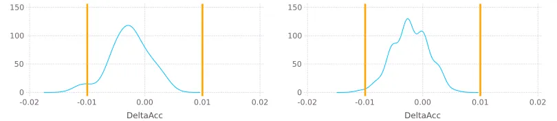
Consider the datasetsquash-unsorted, with the posterior computed by the Bayesian corre-lated t-test for the difference between nbc and aode, as shown in Figure 4. The vertical orange lines mark again the region corresponding to a difference of accuracy of less than 1% (we will clarify the meaning of this region later in the section). In Bayesian analysis, the experiment is summarized by the posterior distribution (in this case a Student distribution). The posterior describes the distribution of the mean difference of accuracies between the two classifiers.
By querying the posterior distribution, we can evaluate the probability of the hypothesis. We can for instance infer the probability that nbc is better/worse than aode. Formally
P(nbc > aode) = 0.165 is the integral of the posterior distribution from zero to infinity or, equivalently, the posterior probability that the mean of the differences of accuracy between nbc and aode is greater than zero. P(aode > nbc) = 1−P(nbc > aode) = 0.835 is the integral of the posterior between minus infinity and zero or, equivalently, the posterior probability that the mean of the differences of accuracy is less than zero.
“prac-DeltaAcc
-0.2 -0.1 0.0 0.1 0.2
pdf rope legend
0 2 4 6 8
Figure 4: Posterior of the Bayesian correlated t-test for the difference betweennbcandaode in the datasetsquash-unsorted.
tically equivalent”. In classification, it is sensible to define that two classifiers whose mean difference of accuracies is less that 1% are practically equivalent. The interval [−0.01,0.01] thus defines a region of practical equivalence (rope) (Kruschke and Liddell, 2015) for clas-sifiers.3 Once we have defined a rope, from the posterior we can compute the probabilities:
• P(nbc aode): the posterior probability of the mean difference of accuracies being practically negative, namely the integral of the posterior on the interval (−∞,−0.01).
• P(nbc=aode): the posterior probability of the two classifiers being practically equiv-alent, namely the integral of the posterior over the rope interval.
• P(nbc aode): the posterior probability of the mean difference of accuracies being practically positive, namely the integral of the posterior on the interval (0.01,∞).
P(nbc=aode) = 0.086 is the integral of the posterior distribution between the vertical lines (the rope) shown in Figure 4 and it represents the probability that the two classifiers are practically equivalent. Similarly, we can compute the probabilities that the two classifiers are practically different, which areP(nbcaode) = 0.788 and P(nbcaode) = 0.126.
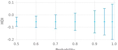
The posterior also shows the uncertainty in the estimate, because the distribution shows the relative credibility of values across the continuum. One way to summarize the uncer-tainty is by marking the span of values that are the most credible and cover q% of the distribution (e.g., q = 90%). These are called theHigh Density Intervals (HDIs) and they are shown in Figure 5 (center) for q= 50,60,70,80,90,95,99.
Thus the posterior distribution equipped with rope:
1. estimates the posterior probability of a sensible null hypothesis (the area within the rope);
2. claims significant differences that also have a practical meaning (the area outside the rope);
Probability
0.5 0.6 0.7 0.8 0.9 1.0
-0.2 -0.1 0.0 0.1
HDI
Figure 5: Posterior HDIs of the Bayesian correlated t-test for the difference between nbc andaode in the datasetsquash-unsorted.
3. represents magnitude (effect size) and uncertainty (HDIs);
4. does not depend on the sampling intentions.
To see that, we apply Bayesian analysis to the critical cases for NHST presented in the previous section. Figure 6 shows the posterior for hepatitis (top), ecoli (left) and iris (right). For hepatitis, all the probability mass is inside the rope and so we can conclude that nbc and aode are practically equivalent: P(nbc =aode) = 1. For ecoli and iris, the probability mass is all in (−∞,0] and so nbc < aode. However, the posterior gives us more information: there is much more uncertainty in theirisdataset. The posteriors thus provide us the same information as the density plots shown in Figures 1–3.
DeltaAcc
-0.015 -0.010 -0.005 0.000 0.005 0.010 0.015
pdf rope
legend
0 100 200 300 400
DeltaAcc
-0.10 -0.05 0.00
pdf rope legend
0 50 100
DeltaAcc
-0.10 -0.05 0.00
pdf rope legend
0 5 10 15 20
Figure 6: Posterior fornbc vs.aode inhepatitis (top),ecoli (left) and iris (right).
obvious way and this is evident from the posterior. Compare these figures with Figure 4, which is similar.
DeltaAcc
-0.03 -0.02 -0.01 0.00 0.01 0.02 0.03 pdf rope legend
0 20 40 60 80
DeltaAcc
-0.05 0.00 0.05
pdf rope legend
0 10 20 30 40 50
Figure 7: Posterior for nbc vs.aode inaudiology (left) andbreast-cancer (right).
Let us repeat the previous analysis for all 54 datasets: Figure 8 reports the posteriors for nbc versusaode in all those cases. Looking at the posteriors, we see that there are 12 cases where aode is practically better than nbc, since all the posterior is outside (to the left of) the rope (in the datasets ecoli, iris, monks1, monks, mushroom, nursey, optdigits, pasture, segment, spambase, credit, owel). There are 6 datasets where nbc and aode are practically equivalent (hayes-roth,hungarian14,hepatitis,labor,wine,yeast), since the entire posterior is inside the rope. We see also that there are no cases where nbc is practically better than aode (posterior to the right of the rope). The posteriors give us information about the magnitude of effect size, practical difference and equivalence, as well as the related uncertainty.
3.2 Sensible automatic decisions
In machine learning, we often need to perform many analyses. So it may be convenient to devise a tool for automatic decision from the posterior. This means that we have to summarize the posterior in some way, with a few numbers. However, we must be aware that every time we do that we go back to that sort of black and white analysis whose limitations have been discussed before. In fact, by summarizing the posterior, we lose information, but we can do so in a conscious way. We have already explained the advantages of introducing a rope, so we can make automatic decisions based on the three probabilities P(nbcaode),
P(nbc = aode) and P(nbc aode). In this way, we lose information but we introduce shades in the black and white thinking. P(nbcaode),P(nbc=aode) andP(nbcaode) are probabilities and their interpretation is clear. P(nbc=aode) is the area of the posterior within the rope and represents the probability thatnbc andaode are practically equivalent.
P(nbc aode) is the area of the posterior to the left of the rope and corresponds to the probability that nbc is practically better than aode. Finally, P(nbc aode) is the area to the right of the rope and represents the probability that aode is practically better than nbc. Since these are the actual probabilities of the decisions we are interested in, in classification, we need not think in terms of Type-I errors to make decisions. We can simply make decisions using these probabilities, which have a direct interpretation—contrarily to
p-values. For instance we can decide
-0.04 -0.03 -0.02 -0.01 0.00 0.01 0.02 0 10 20 30 40 50 zoo
-0.015 -0.010 -0.005 0.000 0.005 0.010 0
50 100 150
yeast
-0.010 -0.005 0.000 0.005 0.010 0.015 0
50 100 150
wine
-0.02 -0.01 0.00 0.01 0.02 0.03 0 10 20 30 40 50 60 white-clover
-0.10 -0.05 0.00 0.05 0 5 10 15 20 waveform
-0.07 -0.06 -0.05 -0.04 -0.03 -0.02 -0.01 0.00 0.01 0 20 40 60 80 owel
-0.3 -0.2 -0.1 0.0 0.1 0
10 20 30
credit
-0.04 -0.02 0.00 0.02 0.04 0 10 20 30 40 50 tae
-0.3 -0.2 -0.1 0.0 0.1 0.2 0 2 4 6 8 squash-unstored
-0.2 -0.1 0.0 0.1 0.2 0.0 2.5 5.0 7.5 10.0 squash-stored
-0.015 -0.010 -0.0050.000 0.005 0.010 0 50 100 150 200 splice
-0.06 -0.04 -0.02 0.00 0.02 0.04 0 10 20 30 40 spect-reordered
-0.06 -0.04 -0.02 0.00 0.02 0
50 100 150
spambase
-0.03 -0.02 -0.01 0.00 0.01 0 20 40 60 80 soybean
-0.04 -0.02 0.00 0.02 0.04 0
10 20 30
40 sonar
-0.10 -0.05 0.00 0.05 0
10 20 30
solar-flare-X
-0.05 0.00 0.05
0 10 20 30 40 solar-flare-m
-0.075 -0.050 -0.025 0.000 0.025 0 10 20 30 40 solar-flare-C
-0.06 -0.04 -0.02 0.00 0.02 0 20 40 60 80 segment
-0.04 -0.02 0.00 0.02 0.04 0 10 20 30 40 50 primary-tumor
-0.10 -0.05 0.00 0.05 0.10 0 5 10 15 20 postoperatie
-0.03 -0.02 -0.01 0.00 0.01 0.02 0 20 40 60 80 pendigits
-0.15 -0.10 -0.05 0.00 0.05 0
50 100 150
pasture-production
-0.050 -0.025 0.000 0.025 0.050 0
10 20 30
page-blocks
-0.06 -0.04 -0.02 0.00 0.02 0
50 100 150
optdigits
-0.06 -0.04 -0.02 0.00 0.02 0
50 100 150
nursery
-0.03 -0.02 -0.01 0.00 0.01 0
100 200 300
400 mushroom
-0.06 -0.04 -0.02 0.00 0.02 0
50 100 150
200 monks
-0.015 -0.010 -0.005 0.000 0.0050.010 0
50 100
150 monks3
-0.15 -0.10 -0.05 0.00 0.05 0 10 20 30 40 monks1
-0.06 -0.04 -0.02 0.00 0.02 0 10 20 30 40 50 60 lymphography
-0.10 -0.05 0.00 0.05 0
10 20 30
lier-disorders
-0.010 -0.005 0.000 0.005 0.010 0.0
0.5 1.0
labor
-0.10 -0.05 0.00 0.05 0 5 10 15 20 25 kr-s-kp
-0.06 -0.04 -0.02 0.00 0.02 0 20 40 60 80 100 iris
-0.02 -0.01 0.00 0.01 0.02 0.03 0 20 40 60 80 ionosphere
-0.10 -0.05 0.00 0.05 0
10 20 30
hypothyroid
-0.010 -0.005 0.000 0.005 0.010 0 100 200 300 400 hepatitis
-0.02 -0.01 0.00 0.01 0.02 0 25 50 75 100 hungarian-14
-0.04 -0.02 0.00 0.02 0.04 0 10 20 30 40 50 cleeland-14
-0.010 -0.005 0.000 0.005 0.010 0.0
0.5 1.0
hayes-roth
-0.06 -0.04 -0.02 0.00 0.02 0.04 0
10 20 30
haberman
-0.05 0.00 0.05 0.10 0.15 0 5 10 15 20 grub-damage
-0.10 -0.05 0.00 0.05 0 5 10 15 20 25 glass
-0.03 -0.02 -0.01 0.00 0.01 0.02 0 10 20 30 40 50 60 eucalyptus
-0.15 -0.10 -0.05 0.00 0.05 0 5 10 15 20 ecoli
-0.02 -0.01 0.00 0.01 0.02 0 20 40 60 80 pima-diabetes
-0.04 -0.03 -0.02 -0.01 0.00 0.01 0.02 0 10 20 30 40 50 60 german-credit
-0.03 -0.02 -0.01 0.00 0.01 0.02 0 20 40 60 80 credit
-0.2 -0.1 0.0 0.1 0.2 0
5 10
contact-lenses
-0.03 -0.02 -0.01 0.00 0.01 0.02 0 10 20 30 40 50 60 cmc
-0.04 -0.02 0.00 0.02 0.04 0 10 20 30 40 50 breast-cancer
-0.02 -0.01 0.00 0.01 0.02 0 20 40 60 80 audiology
-0.04 -0.03 -0.02 -0.01 0.00 0.01 0 20 40 60 80 anneal
Figure 8: Posteriors ofnbc versusaode for all 54 datasets.
2. nbcaodeifP(nbcaode)>0.95;
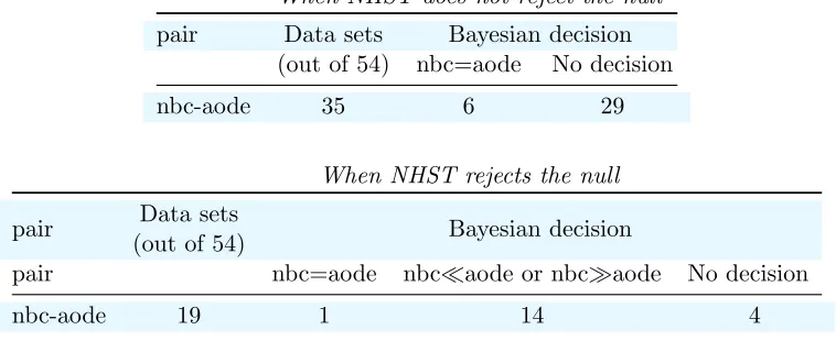
We can also decide with a probability of, for instance, 0.90 or 0.80 (if this is appropriate in the given context). Table 4 compares the Bayesian decisions based on the above rule with the NHST decisions. The NHST fails to reject the null in 35/54 datasets; Bayesian analysis declares the two classifiers equivalent in 6 of such datasets. Conversely, when NHST rejects the null (in 19/54 datasets), the Bayesian analysis declares nbcaode or nbcaode in 14 cases, nbc=aode in 1 case and no decision in 4 cases. Overall, Bayesian analysis allows us to make a decision in 6 + 1 + 14 = 21 datasets, while NHST makes a decision only in 19 cases.
When NHST does not reject the null
pair Data sets Bayesian decision (out of 54) nbc=aode No decision
nbc-aode 35 6 29
When NHST rejects the null
pair Data sets
(out of 54) Bayesian decision
pair nbc=aode nbcaode or nbcaode No decision
nbc-aode 19 1 14 4
Table 4: Results referring to comparisons in which the NHST rejects the null.
Sometimes also in Bayesian analysis it may be convenient to think in terms of errors. We can easily do that by defining a loss function. A loss function defines the loss we incur in making the wrong decision. The decisions we can take are nbcaode (denoted as al), nbcaode (ar), nbc=aode (ac) or none of them (an). Consider for instance the following loss matrix.
al
ac
ar
an
al ac ar
0 20 20
20 0 20
20 20 0
1 1 1
(7)
The first row gives us the loss we incur in decidingal when al is true (zero loss), acis true (loss is 20) and ar is true (loss is 20). Similarly for the second and third rows. The last row is the loss we incur in making no decision. The expected loss can be simply obtained by multiplying the above matrix L for the vector of posterior probabilities of nbcaode, nbc=aode and nbcaode (p = [pl, pc, pr]T), i.e., Lp. The row of Lp corresponding to the lowest loss determines the final decision. Since 0.05·20 = 1, this leads to the same decision rule discussed previously (P(·)>0.95).
3.3 Comparing NHST and Bayesian analysis for other classifiers
The aim of this section is to show that the pattern described above is general and it also holds for other classifiers. The results are presented in two tables. First we report on the cases in which NHST does not reject the null (Tab. 5). Then we report on the comparisons in which the NHST rejects the null (Tab. 6).
The NHST test does not reject the null hypothesis (Tab. 5) in 341/540 comparisons. In these cases the NHST does not make any conclusion: it cannot tell whether the null hypothesis is true4 or whether is false but the evidence is too weak to reject it.
By applying the Bayesian correlated t-test with rope and taking decisions as discussed in the previous section, we can draw more informative conclusions. In 74/341=22% of the rejections failed by NHST, the posterior probability of the rope is larger than 0.95, allowing to declare that the two analyzed classifiers are practically equivalent. In the remaining cases, no conclusion can be drawn with probability 0.95.
The rope thus provides a sensible null hypothesis which can be accepted on the basis of the data. When this happens we conclude that the two classifiers are practically equivalent. This is impossible with the NHST.
When NHST does not reject the null
pair Data sets Bayesian decision
(out of 54) P(rope) >.95 No decision
nbc–aode 35 6 29
nbc–hnb 30 0 30
nbc–j48 27 2 25
nbc–j48gr 27 2 25
aode–hnb 40 6 34
aode–j48 33 6 27
aode–j48gr 35 6 29
hnb–j48 32 3 29
hnb–j48gr 32 3 29
j48–j48gr 50 40 10
total 341 74 267
rates 74/341= 0.22 267/341=0.78
Table 5: Results referring to comparisons in which the NHST correlated t-test does not reject the null.
Let us consider now the comparisons in which NHST claims significance (Tab. 6). There are 199 such cases. The Bayesian estimation procedure confirms the significance of 142/199 (71%) of them: in these cases it estimates either P(lef t) > 0.95 or P(right) >0.95.5 In these cases the accuracy of the two compared classifiers arepractically different. In 51/199 cases (26%) the Bayesian test does not make any conclusion. This means that a sizeable amount of probability lies within the rope, despite the statistical significance claimed by the
4. A point null is however always false, as already discussed.
When NHST rejects the null
pair Data sets
(out of 54) Bayesian decision
pair rope difference no decision
nbc–aode 19 1 14 4
nbc–hnb 24 0 19 5
nbc–j48 27 0 20 7
nbc–j48gr 27 0 21 6
aode–hnb 14 1 6 7
aode–j48 21 1 14 6
aode–j48gr 19 1 13 5
hnb–j48 22 0 17 5
hnb–j48gr 22 0 17 5
j48–j48gr 4 2 1 1
total 199 6 142 51
rates 6/199= 0.03 142/199=0.71 51/199=0.26
Table 6: Results referring to comparisons in which the NHST rejects the null.
frequentist test. In the remaining cases (6/199=3%) the Bayesian test concludes that the two classifiers are practically equivalent (P(rope) > 0.95) despite the significance claimed by the NHST. In this case it draws the opposite conclusion from the NHST.
Summing up, the Bayesian test with rope is more conservative, reducing the claimed significances by 30% as compared with the NHST. The Bayesian test is thus more conserva-tive due to the rope, which constitutes a sensible null hypothesis, while the null hypothesis of the NHST is surely wrong. However counting the detection of practically equivalent classifiers as decisions, the Bayesian test with rope takes more decisions than the NHST (222 vs. 199).
4. Comparing two classifiers on multiple data sets
So far we have discussed how to compare two classifiers on the same data set. In machine learning, another important problem is how to compare two classifiers on a collection of q
different data sets, after having performed cross-validation on each data set.
4.1 The frequentist approach
There is no direct NHST able to perform such statistical comparison, i.e., one that takes as inputs themruns of thek-fold cross-validation differences of accuracy for each dataset and returns as output a statistical decision about which classifier is better in all the datasets. The usual NHST procedure that is employed for performing such an analysis has two steps:
2. perform a NHST to establish if the two classifiers have different performance or not based on these mean differences of accuracy.
For our case study, nbc vs. aode, the mean differences of accuracy in each dataset com-puted from Table 1 are shown in Table 7. We denote these measures generically with
z={z1, . . . , zq} (in our caseq = 54). The recommended NHST for this task is the signed-rank test (Demˇsar, 2006).
Dataset Mean Dif. Dataset Mean Dif. Dataset Mean Dif.
anneal -1.939 audiology -0.261 breast-cancer 0.467
cmc -0.719 contact-lenses 2.000 credit -0.464
german-credit -1.014 pima-diabetes -0.151 ecoli -7.269
eucalyptus -0.790 glass -2.600 grub-damage 4.362
haberman -0.614 hayes-roth 0.000 cleeland-14 -0.625
hungarian-14 -0.069 hepatitis -0.212 hypothyroid -1.683
ionosphere 0.267 iris -3.242 kr-s-kp -0.833
labor 0.000 lier-disorders -1.762 lymphography -1.863
monks1 -10.002 monks3 -0.343 monks -4.190
mushroom -2.434 nursery -4.747 optdigits -3.548
page-blocks 0.583 pasture -10.043 pendigits -0.443
postoperatie 1.333 primary-tumor -0.674 segment -3.922
solar-flare-C -2.776 solar-flare-m -0.688 solar-flare-X -3.996
sonar -0.338 soybean -1.112 spambase -3.284
spect-reordered -1.684 splice -0.699 squash-stored -0.367
squash-unstored -5.600 tae -0.400 credit -16.909
owel -5.040 waveform -1.809 white-clover 0.500
wine 0.143 yeast -0.202 zoo -0.682
Table 7: Mean difference of accuracy (0–100) for each dataset for nbc minus aode
Frequentist signed-rank test
The Wilcoxon signed-rank test is a non-parametric statistical hypothesis test used when comparing two paired samples. The signed-rank test assumes the observations z1, . . . , zq to be i.i.d. and generated from a symmetric distribution. The test is miscalibrated if the distribution is not symmetric. A strict usage of the test should thus include first a test for symmetry. One should run the signed-rank only if “the symmetry test fails to reject the null” (note that, as we discussed before, this does not actually prove that the distribution is symmetric!). However this would make the whole testing procedure cumbersome, requiring also corrections for the test of multiple hypotheses. In the common practice thus the test for symmetry is not performed, and we follow this practice in this paper.
differences. The test statistic is:
t= P
{i:zi≥0}
ri(|zi|) = P 1≤i≤j≤q
t+ij,
whereri(|zi|) is the rank of |zi|and
t+ij =
1 if zi≥ −zj, 0 otherwise.
For instance, let us consider the following two cases z ={−2,−1,4,5} or z ={−1,4,5}, then the statistic is t = 7 and, respectively, t= 5. For a large enough number of samples (e.g., q >10), the statistic under the null hypothesis is approximately normally distributed and in this case the two-sided test is performed as follows:
w= t−
q(q+1) 4 q
q(q+1)(2q+1)−tie 24
,
p= 2(1−Φ(|w|)),
(8)
wherepdenotes thep-value computed w.r.t. Φ, which is the cumulative distribution function of the standard Normal distribution; tie is an adjustment for ties in the data |z|, i.e.,
zi = −zj for some i, j, required by the nonparametric test (Sidak et al., 1999; Hollander et al., 2013), while it is zero in case of no ties.
Being non-parametric, the signed-rank is robust to outliers. It assumes commensura-bility of differences, but only qualitatively: greater differences count more as they top the rank; yet their absolute magnitudes are ignored (Demˇsar, 2006).
4.1.1 Experimental results
If we apply this method to comparenbc vs.aode, we obtain p-value=10−6(the rankt= 162 with no ties and w is −4.8). Since the p-value is less than 0.05, the NHST concludes that the null hypothesis can be rejected and thatnbc andaode are significantly different. Table 8 reports thep-values of all comparisons of the five classifiers. The pairsnbc-aode,nbc-hnb, j48-j48gr are statistically significantly different. Again by applying this black and white mechanism, we encounter the same problems as before, i.e., we do not have any idea of the magnitude of the effect size, the uncertainty, the probability of the null hypothesis, et cetera. The density plot of the data (the mean differences of accuracy in each dataset) for nbc versusaode shows for instance that there are many datasets where the mean difference is small (close to zero), see Figure 9. Instead for j48 versus j48gr, it is clear that the difference of accuracy is very small.
4.2 The Bayesian analysis approach
DeltaAcc
-0.2 -0.1 0.0 0.1
0 10 20 30
DeltaAcc
-0.03 -0.02 -0.01 0.00 0.01
0 100 200 300 400 500
Figure 9: Density plot fornbc versusaode (left) andj48 versus j48gr (right)
Classif. 1 Classif. 2 p-value
nbc aode 0.000
nbc hnb 0.001
nbc j48 0.463
nbc j48gr 0.394
aode hnb 0.654
aode j48 0.077
aode j48gr 0.106
hnb j48 0.067
hnb j48gr 0.084
j48 j48r 0.000
Table 8: p-values for the comparison of the five classifiers.
4.2.1 Nonparametric test
Benavoli et al. (2014) have proposed a Bayesian counterpart of the frequentist sign and signed-rank test, which is based on the Dirichlet process.
Bayesian sign and signed-tank test
Let z denote the scalar variable of interest and z = {z1, . . . , zq} denotes a vector of i.i.d. observations ofz. To derive the Bayesian sign and signed-rank test, we assume a Dirichlet Process (DP) prior on the probability distribution of z. A DP is a distribution over prob-ability distributions such that marginals on finite partitions are Dirichlet distributed. Like the Dirichlet distribution, the DP is therefore completely defined by two parameters: the prior strength s >0 and the prior mean that, for the DP, is a probability measure G0 on
z. If we choose G0 = δz0, i.e., a Dirac’s delta centred on the pseudo-observation z0, the
posterior probability density function of Z has this simple expression:
p(z) =w0δz0(z) +
n
X
j=1
w that are Dirichlet distributed. The model (9) is therefore a posterior distribution of the probability distribution of z and encloses all the information we need for the experimental analysis. We can summarize it in different way. If we compute:
θl=P(z <−r) = q
X
i=0
wiI(−∞,−r)(zi),
θe=P(|z| ≤r) = q
X
i=0
wiI[−r,r](zi),
θr=P(z > r) = q
X
i=0
wiI(r,∞)(zi),
where the indicator IA(z) = 1 if z0 ∈ A and zero otherwise, then we obtain a Bayesian version of thesign testthat also accounts for the rope [−r, r]. In fact,θl, θe, θr are respec-tively the probabilities that the mean difference of accuracy is in the interval (−∞,−r), [−r, r], or (r,∞). Since (w0, w1, . . . , wn)∼Dir(s,1, . . . ,1), it can easily be shown that
θl, θe, θr ∼Dirichlet(nl+sI(−∞,−r](z0), ne+sI[−r,r](z0), nr+sI[r,∞)(z0)), (10) wherenlis the number of observationszithat fall in (−∞,−r],neis the number of observa-tionszithat fall in [−r, r] andnris the number of observationszithat fall in [r,∞), obviously
nl+ne+nr=q. If we neglectsI(−∞,−r](z0), sI[−r,r](z0), sI[r,∞)(z0), then (10) says that the posterior probability of θl, θe, θr is Dirichlet distributed with parameters (nl, ne, nr). The terms sI(−∞,−r](z0), sI[−r,r](z0), sI[r,∞)(z0) are due to the prior. Therefore, to fully specify the Bayesian sign test, we must choose the value of the prior strengthsand where to place the pseudo-observation z0 in (−∞,−r] or [−r, r] or [r,∞). We will return to this choice in Section 4.3. Instead, if we compute
θl= q
X
i=0 q
X
j=0
wiwjI(−∞,−2r)(zj+zi),
θe= q
X
i=0 q
X
j=0
wiwjI[−2r,2r](zj +zi),
θr = q
X
i=0 q
X
j=0
wiwjI(2r,∞)(zj+zi), (11)
then we derive a Bayesian version of thesigned rank test(Benavoli et al., 2014) that also accounts for the rope [−r, r]. This time the distribution ofθl, θe, θr has not a simple closed form but we can easily compute it by Monte Carlo sampling the weights (w0, w1, . . . , wn)∼
Dir(s,1, . . . ,1). Also in this case we must choose s, z0, see Section 4.3.
the distribution from data). This is another advantage of the Bayesian estimation approach w.r.t. the frequentist null hypothesis tests (Benavoli et al., 2014).
4.2.2 Experiments
Let us start by comparing nbc vs. aode by means of the Bayesian sign-rank tests without rope (r= 0). Hereafter we will choose the prior parameter of the Dirichlet as s= 0.5 and
z0 = 0; we will return to this choice in Section 4.3. Since without rope θr = 1−θl, we have only reported the posterior of θl (denoted as “Pleft”) that represents the probability thataode is better thannbc. The samples of the posteriors are shown in Figure 10: this is simply the histogram of 1500000 samples ofθl generated according to (11). For all samples, it results inθl greater than 0.5 and soθr= 1−θl. So we can conclude with probability ≈1 that aode is better than nbc. We can in fact think about the comparison of two classifiers as the inference on the bias (θl) of a coin. In this case, all the 1500000 sampled coins from the posterior have a bias that is greater than 0.5 and, therefore, all the coins are always biased towardsaode (which is then preferable to nbc).
This conclusion is in agreement with that derived by the frequentist sign-rank test (very small p-value, see Table 8).
Pleft
0.5 0.6 0.7 0.8 0.9 1.0
0 500 1000 1500
Figure 10: Posterior for nbc vs. aode for the Bayesian sign-rank test.
aode
0.0 0.5 1.0 1
200
50 100 150 Count
0.0 0.2 0.4 0.6 0.8
rope
nbc
0.0 0.1 0.2 0.3
1 100
50 Count
0.0 0.2 0.4 0.6 0.8
rope
1 25 50 75 100 Count rope
aode nbc
Figure 11: Posterior for nbc vs. aode for the Bayesian sign-rank test.
probable than “aode” and “nbc” together; the region at the left of the triangle corresponds to the case where “nbc” is more probable than “aode” and “rope” together. Hence, if all the points fall inside one of these three regions, we conclude that such hypothesis is true with probability ≈ 1. Looking at Figure 11 (bottom), it is evident that the majority of cases support aode more than rope and definitively more than nbc. We can quantify this numerically by counting the number of points that fall in the three regions, see first row in Table 9. aode is better in 90% of cases, while rope is selected in the remaining 10%. We can therefore conclude with probability 90% that aode is practically better than nbc. Table 9 reports also these probabilities for the other comparisons of classifiers computed using 1500000 Monte Carlo samples. We conclude that hnb is practically better than nbc with probability 0.999; aode and hnb are equivalent with probability 0.95; aode is better thanj48 and j48gr with probability 0.9;hnb is better thanj48 andj48gr with probability greater than 0.95 and finally j48 and j48gr are practically equivalent. These conclusions are in agreement with the data.
The computational complexity of the Bayesian sign-rank test is low. The comparison of two classifiers (based on 1500000 samples) takes less than one second on a standard computer.
4.3 Choice of the prior
In the previous section, we have selected the prior parameters of the Dirichlet process as
500 1500 1000 1 Count rope j48gr j48 10 50 30 1 20 40 Count rope j48gr hnb 30 20 10 60 40 1 50 Count rope j48 hnb 10 50 30 1 20 40 Count rope j48gr aode 10 50 30 1 20 40 Count rope j48 aode 10 50 30 1 20 40 Count rope hnb aode 30 20 10 60 40 1 50 Count rope j48gr nbc 30 20 10 60 40 1 50 Count rope j48 nbc 30 20 10 60 40 1 50 Count rope hnb nbc
Figure 12: Posterior for nbc vs.aode for Bayesian sign-rank test.
equivalent to that of one pseudo-observation that is located inside the rope (Benavoli et al., 2014). How are the inferences sensitive to this choice? For instance, we can see how the probabilities on Table 9 would change based on z0. We have considered two extreme cases
z0 = −∞ and z0 = ∞ and reported these probabilities in Table 10 and 11 (this is an example of robust Bayesian analysis (Berger et al., 1994)). It is evident that the position of z0 has only a minor effect on the probabilities. We could have performed this analysis jointly by considering all the possible Dirichlet process priors obtained by varying z0 ∈R.
Classif. 1 Classif. 2 left rope right
nbc aode 0.000 0.103 0.897
nbc hnb 0.000 0.001 0.999
nbc j48 0.228 0.004 0.768
nbc j48gr 0.182 0.002 0.815
aode hnb 0.001 0.956 0.042
aode j48 0.911 0.026 0.063
aode j48gr 0.892 0.035 0.073
hnb j48 0.966 0.015 0.019
hnb j48gr 0.955 0.020 0.025 j48 j48gr 0.000 1.000 0.000
Table 9: Probabilities for the ten comparisons of classifiers. Left and right refer to the columns Classif. 1 (left) and Classif. 2 (right).
Classif. 1 Classif. 2 left rope right
nbc aode 0.000 0.112 0.888
nbc hnb 0.000 0.001 0.999
nbc j48 0.262 0.004 0.734
nbc j48gr 0.213 0.003 0.784
aode hnb 0.002 0.961 0.037
aode j48 0.922 0.024 0.053
aode j48gr 0.906 0.033 0.061
hnb j48 0.971 0.014 0.016
hnb j48gr 0.961 0.018 0.021 j48 j48gr 0.000 1.000 0.000
Table 10: Probabilities for the ten comparisons of classifiers with z0 =∞. Left and right refer to the columns Classif. 1 (left) and Classif. 2 (right).
4.3.1 Hierarchical models
Classif. 1 Classif. 2 left rope right
nbc aode 0.000 0.096 0.904
nbc hnb 0.000 0.001 0.999
nbc j48 0.201 0.004 0.795
nbc j48gr 0.159 0.002 0.839
aode hnb 0.001 0.950 0.049
aode j48 0.892 0.028 0.080
aode j48gr 0.872 0.037 0.091
hnb j48 0.957 0.017 0.027
hnb j48gr 0.944 0.022 0.034 j48 j48gr 0.000 1.000 0.000
Table 11: Probabilities for the ten comparisons of classifiers with z0 =−∞. Left and right refer to the columns Classif. 1 (left) and Classif. 2 (right).
the mean difference of accuracy for each dataset ¯xi; (2) perform a NHST to establish if the two classifiers have different performance or not based on these mean differences of accuracy. This discards two pieces of information: the correlation ρ and sample standard deviation ˆσiin each dataset. The standard deviation is informative about the accuracy of ¯xi as an estimator of µi. The standard deviation can largely vary across data sets, as a result of each data set having its own size and complexity. The aim of this section is to present an extension of the Bayesian correlated t-test that is able to make inference on multiple datasets and at the same time to account for all the available information (mean, standard deviation and correlation). In Bayesian estimation, this can be obtained by defining a hierarchical model (Corani et al., 2017). Hierarchical models are among the most powerful and flexible tools in Bayesian analysis.
Bayesian hierarchical correlated t-test
The hierarchical correlated t-test is based on following hierarchical probabilistic model:
xi ∼M V N(1µi,Σi), (12)
µ1...µq∼t(µ0, σ0, ν), (13)
σ1...σq ∼unif(0,σ¯). (14)
be drawn from a high-level Student distribution with mean µ0, variance σ20 and degrees of freedom ν. The choice of a Student distribution at this level of the hierarchical model enables the model to robustly deal with data sets whose µi’s are far away from the others (Gelman et al., 2014; Kruschke, 2013). Moreover the heavy tails of the Student make more cautious the conclusions drawn by the model.
The hierarchical model assigns to the i-th data set its own standard deviation σi, as-suming theσi’s to be drawn from a common distribution, see Equation (14). In this way it realistically represents the fact the estimates referring to different data sets data sets have different uncertainty. The high-level distribution of theσi’s is unif(0,σ¯), as recommended by Gelman (2006), as it yields inferences which are insensitive to ¯σ, if ¯σ is large enough. To this end we set ¯σ= 1000·¯s(Kruschke, 2013), where ¯s=Pq
iσˆi/q.
We complete the model with the prior on the parametersδ0,σ0 andν of the high-level distribution. We assumeδ0 to be uniformly distributed within 1 and -1. This choice works for all the measures bounded within±1, such as accuracy, AUC, precision and recall. Other type of indicators might require different bounds.
For the standard deviation σ0 we adopt the priorunif(0,s¯0), with ¯s0 = 1000sx¯, where
s¯x is the standard deviation of the ¯xi’s.
As for the priorp(ν) on the degrees of freedom, there are two proposals in the literature. Kruschke (2013) proposes an exponentially shaped distribution which balances the prior probability of nearly normal distributions (ν >30) and heavy tailed distributions (ν <30). We re-parameterize this distribution as a Gamma(α,β) with α=1, β= 0.0345. Ju´arez and Steel (2010) proposes instead p(ν) = Gamma(2,0.1), assigning larger prior probability to normal distributions.
We have no reason for preferring a prior over another, but the hierarchical model shows some sensitivity on the choice of p(ν). We model this uncertainty by representing the coefficientsαandβ of the Gamma distribution as two random variables (hierarchical prior). In particular we assume p(ν) = Gamma(α, β), with α ∼ unif(α,α¯) and β ∼ unif(β,β¯), setting α=0.5, ¯α=5, β=0.05, ¯β=0.15. The simulations in (Corani et al., 2017) show that the inferences of the model are stable with respect to perturbations ofα, ¯α,β, and ¯β, and that the resulting hierarchical generally fits well the experimental data.
These considerations are reflected by the following probabilistic model:
ν ∼Ga(α, β), (15)
α∼unif(α, α), (16)
β ∼unif(β, β), (17)
µ0 ∼unif(−1,1), (18)
σ0∼unif(0,σ¯0). (19)
A further merit of the hierarchical model is that it jointly estimates the µi’s while the existing methods estimate independently the difference of accuracy on each data set using the ¯xi’s. The consequence of the joint estimation performed by the hierarchical model is that shrinkage is applied to the ¯xi’s. The hierarchical model thus estimates the µi’s more accurately than the ¯xi’s adopted by the other tests. This result is valid under general assumptions, such as a severe misspecification between the high-level distributions of the true generative model and of the fitted model (Corani et al., 2017). By applying the rope on the posterior distribution of the µi’s and the µ0 in a similar way to what discussed for the Bayesian correlated t-test, the model is able to detect equivalent classifiers and to claim significances that have a practical impact.
4.3.2 Experiments
In the experiments, we have computed the posterior ofµ0, σ0, ν for the ten pairwise compar-isons between the classifiers nbc,aode,hnb,j48 and j48gr. As inference we have computed the prediction on the next (unseen) dataset, which is formally equivalent to the inference computed by the Bayesian signed-rank test. For instance, for nbc vs. aode, we have com-puted the probabilities that in the next datasetnbcis better thanaode(θr),nbcis equivalent toaode (θe), aode is better thannbc (θl). This is the procedure we have followed:
1. we have sampledµ0, σ0, ν from the posteriors of these parameters;
2. for each sample of µ0, σ0, ν we have defined the posterior of the mean difference of accuracy on the next dataset, i.e.,t(µnext;µ0, σ0, ν);
3. fromt(µnext;µ0, σ0, ν) we have computed the probabilitiesθl(integral on (−∞, r]), θe (integral on [−r, r]) andθr (integral on [r,∞)).
1 20
10 15 25
5 Count
rope
aode nbc
Figure 13: Posterior ofnbc versusaode for all 54 datasets.
Classif. 1 Classif. 2 left rope right
nbc aode 0 0.28 0.72
nbc hnb 0 0 1
nbc j48 0.2 0.01 0.79
nbc j48gr 0.15 0.01 0.84
aode hnb 0 1 0
aode j48 0.46 0.51 0.03
aode j48gr 0.41 0.56 0.03
hnb j48 0.91 0.07 0.02
hnb j48gr 0.92 0.05 0.03
j48 j48gr 0 1 0
Table 12: Probabilities for the ten comparisons of classifiers. Left and right refer to the columns Classif. 1 (left) and Classif. 2 (right).
4.4 Choice of the hyper-priors parameters
The choice of of the hyper-priors parameters can be critical in Bayesian hierarchical models. We have conducted a sensitivity analysis by using different constants in the top-level gamma and uniform distributions, to check whether they have any notable influence on the resulting posterior distribution. Whether all gamma/uniform distributions are assumed, the results are essentially identical. More details about this sensitivity analysis are reported in Corani et al. (2017). This means that for the hierarchical model inferences and decisions are stable w.r.t. the choice of the hyper-parameters.
4.5 Bayesian signed rank or hierarchical model?
classifiers? In our opinion, the hierarchical model is preferable because it takes as inputs the
mruns of thek-fold cross-validation results for each dataset and so it makes inference about the mean difference of accuracy between two classifiers in thei-th dataset (µi) by exploiting all available information: the sample mean (¯xi), the variability of the data (sample standard deviation ˆσi) and the correlation due to the overlapping training set (ρ). Conversely, the Bayesian signed rank only considers ¯xi. On the other hand, the hierarchical model is slower than the Bayesian signed rank. In machine learning, we often need to run statistical tests hundreds of times for instance for features selection or algorithms racing and, in this case, it is more convenient to use a light test as the Bayesian signed rank.
5. Comparisons of multiple classifiers
Another important problem with NHST is the issue of multiple hypothesis testing. Con-sidering the results in Table 8, which reports the p-values for the comparison of the five classifiers obtained by the Wilcoxon signed-rank test. From the p-values, we concluded that “nbc was found significantly better thanaode and hnb, and algorithms j48 and j48gr were significantly different, while there were no significant differences between other pairs”. When many tests are made, the probability of making at least one Type 1 error in any of the comparisons increases. One of the most popular fixes to this problem is the Bonferroni correction. The Bonferroni correction adjusts thep-value at which a test is evaluated for sig-nificance according to the number of tests being performed. More specifically, the adjusted
p-value is calculated as the originalp-value divided by the number of tests being performed. Implicitly, Bonferroni’s correction assumes that these test statistics are independent. So in our current example an overall desired significance level of 0.05 would translate into individual tests each using a p-value threshold of 0.05/10 = 0.005 (we are performing 10 comparisons). In this case, this would not change our previous sections, since all significant
p-values were less than 0.005. The Bonferroni correction reduces false rejections but it also increases the number of instances in which the null is not rejected when actually it should have been. Thus, the Bonferroni adjustment can reduce the power to detect an important effect. Motivated by this issue of the Bonferroni correction, researchers have proposed al-ternative procedures. The goal of these methods typically is to reduce the family-wise error rate (that is, the probability of having at least one false positive) without sacrificing power too much. A natural way to achieve this is by considering the dependence across tests (Westfall et al., 1993).
How do we manage the problem of multiple hypothesis testing in Bayesian analysis? Paraphrasing Gelman et al. (2012): “in Bayesian analysis we usually do not have to worry about multiple comparisons. The reason is that we do not worry about Type I error, because the null hypothesis is hardly believable to be true.” How does Bayesian Analysis mitigate false alarms? Gelman et al. (2012) suggest using multilevel analysis (in our case a hierarchical Bayesian model on multiple classifiers). Multilevel models perform partial pooling; they shift estimates toward each other. This means that the comparisons of the classifiers are more conservative, in the sense that intervals for comparisons are more likely to include zero. This may be a direction to pursue in future research. In this paper, we instead mitigate false alarms through the rope. The rope mitigates false alarms because it decreases the asymptotic false alarm rate (Kruschke, 2013).
6. Software and available Bayesian tests
All the tests that we have presented in this paper are available in R andPython code at
https://github.com/BayesianTestsML/tutorial/.
Moreover, the code that is necessary to replicate all the analyses we performed in this paper is also available at the above URL in form of Ipython notebooks (implemented in Python and Julia). The software is open source and that can be freely used, changed, and shared (in modified or unmodified form).
Machine learning researchers may be interested in using other Bayesian tests besides the ones we have discussed in this paper. General Bayesian parametric tests can be found in Kruschke (2015) (together with R code) and also in Gelman et al. (2013). We have specialized some of these tests to the case of correlated data, such as the Bayesian correlated t-test (Corani and Benavoli, 2015) discussed in Section 3. We have also implemented several Bayesian nonparametric tests for comparing algorithms: Bayesian rank test (Benavoli et al., 2015b), Friedman test (Benavoli et al., 2015a) and tests that account for censored data (Mangili et al., 2015). Finally, we have developed an extension of the Bayesian sign test to compare algorithms taking into account multiple measures at the same time (accuracy and computational time for instance) (Benavoli and Campos, 2015). For the analysis of multiple data sets, another approach has been proposed by Lacoste et al. (2012) that models each data set as an independent Bernoulli trial. The two possible outcomes of the Bernoulli trial are the first classifier being more accurate than the second or vice versa. This approach yields the posterior probability of the first classifier being more accurate than the second classifier on more than half of theq data sets. A shortcoming is that its conclusions apply only to the q available data sets without generalizing to the whole population of data sets
7. Conclusions
In this paper, we have discussed how Bayesian analysis can be employed instead of NHST. In particular, we have presented three Bayesian tests: Bayesian correlated t-test, Bayesian signed rank test and a Bayesian hierarchical model that can be used for comparing the performance of classifiers and that solve the drawbacks of the frequentist tests. All the code of these tests is freely available and so researchers can already use these tests for their analysis. In this paper, we have mainly discussed the use of Bayesian tests for comparing the performance of algorithms. However, in machine learning, NHST statistical tests are also employed inside the algorithms. For instance, nonparametric tests are used in racing algorithms, independence tests are used to learn the structure of Bayesian networks, etcetera. Bayesian tests can be used to replace all NHST tests because of their advantages (for instance, Bayesian tests can assess whether two algorithms are similar through the use of the rope (Benavoli et al., 2015a)).
Acknowledgements
Research partially supported by the Swiss NSF grant no. IZKSZ2 162188.
References
Murray Aitkin. Posterior Bayes factors. Journal of the Royal Statistical Society. Series B (Methodological), pages 111–142, 1991.
M.J. Bayarri and James O Berger. Hypothesis Testing and Model Uncertainty. InBayesian Theory and Applications, pages 365–394. OUP Oxford, 2013.
Alessio Benavoli and Cassio P. Campos. Advanced Methodologies for Bayesian Networks: Second International Workshop, AMBN 2015, Yokohama, Japan, November 16-18, 2015. Proceedings, chapter Statistical tests for joint analysis of performance measures. Springer International Publishing, Cham, 2015.
Alessio Benavoli, Francesca Mangili, Giorgio Corani, Marco Zaffalon, and Fabrizio Ruggeri. A Bayesian Wilcoxon signed-rank test based on the Dirichlet process. In Proceedings of the 30th International Conference on Machine Learning (ICML 2014), pages 1–9, 2014.
Alessio Benavoli, Giorgio Corani, Francesca Mangili, and Marco Zaffalon. A Bayesian non-parametric procedure for comparing algorithms. In Proceedings of the 31th International Conference on Machine Learning (ICML 2015), pages 1–9, 2015a.
Alessio Benavoli, Francesca Mangili, Fabrizio Ruggeri, and Marco Zaffalon. Imprecise Dirichlet process with application to the hypothesis test on the probability that X≤Y. Journal of Statistical Theory and Practice, 9(3):658–684, 2015b.
Alessio Benavoli, Giorgio Corani, and Francesca Mangili. Should we really use post-hoc tests based on mean-ranks? Journal of Machine Learning Research, 17(5):1–10, 2016.