Estimation of Volatility and Correlation with Multivariate Generalized Autoregressive Conditional Heteroskedasticity Models: An Application to Moroccan Stock Markets

Issues

ISSN: 2146-4138

available at http: www.econjournals.com

International Journal of Economics and Financial Issues, 2017, 7(2), 384-396.

384

Estimation of Volatility and Correlation with Multivariate

Generalized Autoregressive Conditional Heteroskedasticity

Models: An Application to Moroccan Stock Markets

Yassine Belasri

_{*, Rachid Ellaia}

_*

1_{Laboratory of Study and Research in Applied Mathematics, LERMA, Mohammed V University, Agdal, Morocco,} 2_Mohammadia School of Engineering, BP 765, Rabat, Agdal, Morocco. *Email: [email protected], [email protected]

ABSTRACT

Volatility and correlation are important metrics of risk evaluation for financial markets worldwide. The latter have shown that these tools are varying

over time, thus, they require an appropriate estimation models to adequately capture their dynamics. Multivariate generalized autoregressive conditional

heteroskedasticity (GARCH) models were developed for this purpose and have known a great success. The purpose of this article is to examine the performance of multivariate GARCH models to estimate variance covariance matrices in application to 10 years of daily stock prices in Moroccan stock markets. The estimation is done through the most widely used multivariate GARCH models, dynamic conditional correlation (DCC) and Baba,

Engle, Kraft and Kroner (BEKK) models. A comparison of estimated results is done using multiple statistical tests and with application to volatility

forecast and value at risk (VaR) calculation. The results show that BEKK model performs better than DCC in modeling variance covariance matrices

and that both models failed to adequately estimate VaR.

Keywords: Volatility, Correlation, Multivariate Generalized Autoregressive Conditional Heteroskedasticity, Diagonal Baba; Engle; Kraft and Kroner, Dynamic Conditional Correlation, Stock Markets, Morocco

JEL Classifications: C3, E44, G1

1. INTRODUCTION

Asset pricing, risk assessment, and portfolio management are

undoubtedly the most important activities in financial institutions.

Institutions are concerned by measuring and forecasting changes in their portfolio values according to different market conditions.

The tool that practitioners and researchers use to quantify these changes is volatility. Volatility is defined as variation in an asset

prices over a period of time. Correlation is also an important tool that measures co-movements between multiple assets.

Financial markets worldwide have shown that volatility is varying over time. A number of researchers studied this phenomenon, for

example: Officer (1973) showed that volatility changes are related macroeconomic variables, Black (1976) and Christie (1982) argued that financial leverage partly explains it, Merton (1980)

among others1 _{related macroenomic volatility to interest rates.}

1 Pindyck (1984), Bollerslev et al. (1988).

Volatility is not observable and then should be estimated. In 1982,

Engle introduced the autoregressive conditional heteroskedasticity

(ARCH) model. The AR part is due to the fact that these models are autoregressive models in squared returns. The conditional part comes from the fact that next period volatility is conditional

on information set until this period. Heteroscedasticity means non constant volatility. As there were no other methods available

before, Engle’s ARCH model contributed significantly to financial

econometrics by allowing conditional variances to change over

time. The primary descriptive tool was the rolling standard

deviation.

In 1986, Bollerslev developed a generalization of the ARCH

model. He built a more general concept of Engle’s ARCH model by including q lags of the conditional variance (denoted generalized

logarithm of the variance instead of modeling the variance directly,

Runkle (1993) and his GJR-GARCH model which is an extension

of the standard GARCH(P,Q), it includes asymmetric terms in

the conditional variance of equities. Other models also exist in literature, we cite TARCH model (Rabemananjara and Zakoian [1993]) and APARCH of Ding and Granger (1996).

Although Univariate GARCH family models were a great

invention in the financial econometrics, they are unable to estimate correlations when multiple assets are involved. For example, the main problem in portfolio selection, which is defining the optimal

weights of the underlying asset returns, depends on correlations

estimation. Another example is pricing of derivatives contracts

based on multiple underlying assets that requires correlations estimation. Actually, it is commonly accepted that assets volatilities move together, consequently, it is important to capture adequately the interdependence’s between different assets in a portfolio. Multivariate GARCH models were developed to respond to these needs. However, these models face many challenges to adequately capture variances and covariance’s dynamics.

From one hand, the number of parameters of a model may explode when the number of assets increases, this causes complexities

problems in computation and interpretation of parameters, also, reducing the number of parameters should not impact the quality of the model in capturing variances and covariance’s dynamics. From

the other hand, and as stated in Merton (1972), Roll (1977), and Jobson and Korkie (1989), among others, multivariate GARCH models should insure the positive-definiteness of the resulted variance covariance’s matrix. This requirement may appear to be satisfied, as by definition, the variance of random variables is positive. But, there are many possibilities were covariance matrix can be non-positive definite, for example in case assets exhibit non constant volatility or in case of the use of insufficient observation in estimation. For the positive definiteness can be achieved in general in two ways. The first one is constructing a model in a way that the resulted matrix is definite positive, the second one is imposing condition in a way that the computed variance covariance matrix is positive definite, the second alternative is hard to apply in practice.

Over the past two decades, a considerable literature has been developed around multivariate GARCH models. The first one was introduced by Bollerslev et al. (1988), the VEC model. It had the advantage that its coefficients can be directly interpreted. But this model is very general and difficult to implement in practice, it does not guarantee the positive definiteness of the variance covariance’s matrix, also it suffers from high dimensionality of parameters to estimate. Bollerslev et al. (1988) proposed diagonal VEC model which is a simplified version of the VEC model. It reduced the number of parameters to estimate by assuming that model coefficients are diagonal matrices, it guarantees also the positive definiteness of the variance covariance’s matrix, but because of element of the covariance matrix depends on past observations of itself, it does not

capture interactions between different variances and covariance’s.

Engle and Kroner (1995) proposed the Baba, Engle, Kraft and

Kroner (BEKK)2 _{model which can be viewed as a restricted version}

2 BEKK named after model authors: Baba, Engle, Kraft, and Kroner.

of the VEC model. It has the advantage that variance-covariance

matrix is definite positive by construction, but the interpretation of

model parameters is not easy, also, like the VEC model, it suffers

from high dimensionality problem. Many other simplifications

of the full BEKK model were added to the literature, we cite the

Diagonal and Scalar BEKK models. These two models reduced the

number of parameters to estimate in comparison to the VEC model.

To overcome the problem of high number of parameters to estimate in the previously cited models, Engle et al. (1990) introduced another approach of MGARCH models. These models are called

factor GARCH models. It is assumed that the observations are generated by underlying factors that are conditionally

heteroskedastic and possess a GARCH-type structure. The number

of factors to be modeled can be much smaller than the number of assets which make these models feasible even for high number

of assets. Alexander (2001) developed the orthogonal-GARCH model. This model is computationally simple. It is based on only the first few components of the entire risk factors. This model

reduced the number of parameters to estimate but like the BEKK

model, parameters are difficult to interpret.

Another approach in MGARCH is modeling the conditional variances and correlations instead of modeling the conditional

covariance matrix directly. The conditional covariance matrix is

decomposed into conditional standard deviations and a correlation

matrix. Bollerslev (1990) introduced the first category of these

models, namely the constant conditional correlation (CCC) model.

Conditional correlation matrix is assumed to be time invariant in

this model which makes it computationally attractive. It insures

the positive definiteness of the variance-covariance matrix and

reduces the number of parameters to estimate. But the assumption

that conditional correlation matrix is constant is unrealistic in

reality.

Engle (2002) suggested a generalization of the CCC model by letting the conditional correlation matrix to be time varying. This model is called dynamic conditional correlation model (DCC). There has been a growing interest to this model since

its introduction and it has a central role in dynamic correlation modeling. Firstly, the number of parameters to estimate is smaller

comparing to BEKK model, also, it decreases the complexity of

the computation in case of a high number of assets, because the estimation is done into two steps. Also, one main advantage of this

model is that it guarantees the positive definiteness of variance covariance matrix at each point in time.

The purpose of this article is to empirically study, based on the

theory of multivariate GARCH models, co movements between assets in Moroccan stock markets. We selected stocks that have the longest and continuous available historical prices. We choose also two of the most widely used multivariate GARCH models,

diagonal BEKK and DCC. Models order selection is done through the appropriate statistical tests. Once the models are estimated,

we study the quality of the estimation and we use the obtained results in calculating the value at risk (VaR) and volatility forecast.

This will allow us to compare between the estimated models in

386

This paper is organized as follows; next section presents a

theoretical framework of Univariate GARCH, diagonal BEKK

and DCC models, the third section presents data used and the

empirical results before concluding in the last section.

2. THEORETICAL FRAMEWORK

2.1. Univariate GARCH Models

Define σ_t as the standard deviation, S_t the price and r_t the excess return of an asset on day t. (ϵ_t) is an i.i.d sequence. The excess return on t is defined as:

t t-1 S r=ln S    

  (1)

Engle (1982) introduced the ARCH(p) model. The variance is

estimated based on the past p observations, less weights is given

to older observations. The model equation is established as below:

p

2 2

t i t i

i=1 = r ₋

σ ω +

∑

The simplest ARCH model is ARCH(1). Equation becomes:

2 2

t= + r1 t 1−

σ ω α (3)

To insure that σ is positive, ω and α should both be >0. Also, for stationary purposes, α should be <1. In this model, large values of

r_t−1 imply high values of σ_t. Large values of r_t−1 mean high volatility

at t−1. Consequently, in an ARCH (1) model, high volatility cluster may cause more volatility clustering. Bollesrev (1986) suggested

a generalization of the ARCH(P) model that features this behavior, the GARCH(P,Q) model, the current level of volatility depends not

only of P lags of excess returns, but also from Q lags of variances. The equation of GARCH(P,Q) is:

p q

2 2 2

t i t i i t i

i=1 i=1

= + r +− −

σ ω

∑

∑

α₁, α₂,…, α_p, β₁…, β_q are positive, ω > 0 and: max(p,q) _{i i}

i 1

<1 =

α β

∑

stationary.

GARCH model lags p and q can be selected using the Akaike information criterion (AIC) and Bayesian information criterion (BIC). AIC and BIC allow us to choose GARCH model

that best fit our data. AIC and BIC formulas will be detailed later

in this article.

GARCH coefficients can be estimated using the maximum likelihood. Another way to check the goodness of fit of a GARCH

model is checking the autocorrelation of standardized residuals using the autocorrelation function (ACF). If the ACF shows a little autocorrelation of the standardized residuals, then the model

is well fitted. This means that most of the autocorrelation was explained by the model.

2.2. Multivariate GARCH

When we move from a scalar r to a d dimensional one, the variance

σ become a d × d covariance matrix process ∑. The multivariate GARCH model defines r_t as:

r =H_{t t}

1

2 t

η (5)

Where, r_t is a N × 1 vector of excess returns of N assets with

E(r_t) = 0 and η_t is an i.i.d vector error with ' t t

E=[η η]. H_t is the

conditional covariance matrix of r_t (N × N matrix).

The objective of multivariate GARCH process is to estimate Ht. Many approaches have been developed to model it; we will use two of them in the present article. The first approach estimates the covariance matrix directly, it includes VEC and BEKK models. The second one models the conditional variances and correlations

instead of directly modeling H_t, this class of models includes CCC

and DCC.

Bollerslev et al. (1988) introduced the VEC (P,Q) model, it is a

generalization of the Univariate GARCH model, its equation is

defined as below:

( )

(

)

( )

t j t j t j j t j

j=1 j=1

vech H =c+ A vech

∑

∑

Where, vech(.) (Vech is an abbreviation for vector-half) is an operator that creates a column vector whose elements are the

stacked columns of the lower triangular elements of matrix, c is an N(N + 1)/2 × 1 vector and A_j and B_j are N(N + 1)/2 × N(N +

1)/2 matrices of parameters. But the VEC model presents many

disadvantages, for example it does not guaranty the positive definiteness of H_t, also, the number of parameters to estimate is very large, it is equal to: (p + q)(N(N + 1)/2)2_{+(N + 1)/2.}

Bollerslev et al. (1988) presented the diagonal VEC model, it is a simplified version of the initial VEC model that guaranty the positive definiteness of H_t with (p + q + 1)N(N + 1)/2 parameters. It assumes that A_j and B_j are diagonal matrices. But this version of the VEC model is still computationally demanding.

Engle and Kroner (1995) introduced a restricted version of the VEC model, it is called BEKK model. This model equation is

written as below:

p K q K

' ' ' '

t kj t j t j kj kj t j kj

j=1 k=1 j 1 k=1

H =CC A ₋ A B H B₋

= −

+

∑∑

∑∑

Where, A_kj, B_kj are N × N parameter matrices and C is N × N lower triangular matrix. This model economizes the number of

parameters to estimate and allow cross dynamics of conditional

covariance’s. If we set B = AD, where D is a diagonal matrix,

equation 7 can be interpreted as modeling conditional variances

and covariance’s. The diagonal BEKK model is a simplified

version of BEKK where matrices A and B are considered as

diagonal. Equation B = AD is satisfied in this model. BEKK model insure the positive definiteness of H_t.

The second approach that we are interested at in the present article are the ones that models conditional covariance’s matrix indirectly,

it has the form bellow:

Where, (1/2) (1/2)

t 1 N

D =diag (h t ,...,h t ) is diagonal matrix of

conditional variances and Γ_t is the conditional correlation matrix

of r_t, Γ_t = (ρ_ij,t) is positive, definite and symmetric with ρ_ii = 1 ∀ i, each h_jt is modeled by an Univariate GARCH process.

Bollerslev (1990) proposed the CCC model where Γ_t is assumed

to be constant. This model simplifies the estimation. However, assuming that Γ_t is constant is not realistic in practice.

Engle (2002) introduced the DCC model by letting Γ_t to be time

varying. It is defined as:

1 1

2 2

t = diag Qt Q diag Qt t

− −

   

Γ _ _ _ _

    (9)

Where, Q = 1- - Q+ u u + Qt

(

)

positive definite matrix. u_t is the standardized residuals matrix. Q

is the N × N unconditional variance matrix of u_t and α and β are non-negative scalar parameters with α and β < 1.

3. EMPIRICAL RESULTS

3.1. Data Description

Data we employed in this study are daily observations on stock

returns. We used daily data to ensure large number of observations

to adequately fit models. We choose stocks that have the longest

and continuous available historical prices in Casablanca Stock

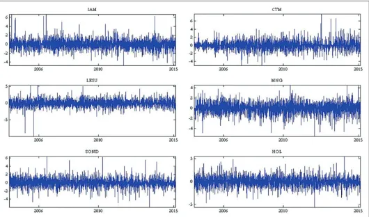
exchange market. Data series start from date 22/02/2004 to 20/10/2015 providing a total of 2749 observations for each series. Six equities have been selected, they are labeled: IAM, CTM, LESU, MNG, SOND and HOL. Our data were retrieved from Thomson Reuters databases and all calculations were done

using Matlab software. Table 1 presents descriptive statistics of our series.

Figure 1 plots daily returns. It can be seen from this figure that our series volatilities don’t keep constant over time, also high returns tend to be followed by high returns and low returns tend to be close with low returns, this is the volatility clustering property.

Kurtosis3 _{calculated for our series presented in Table 1 are >3,}

indicating that they have fat tailed distributions. The skewness4 _are different from zero meaning that they are asymmetric distributions.

The computed statistics of Jarque-Berra normality test5 _{are all}

greater that the critical value (in our case it is = 5.9716) which

rejects the hypothesis of normality of our daily returns.

3 Kurtosis gives a measure of the thickness in the tails of a probability density function. For a normal distribution the kurtosis is 3. A fat-tailed or

thick-tailed distribution has a value for kurtosis that exceeds 3. This is called

leptokurtosis.

4 Skewness gives a measure of how symmetric the observations are about the

mean. For a normal distribution the skewness is 0. A distribution skewed

to the right has positive skewness and a distribution skewed to the left has negative skewness.

5 Jarque-Berra is a test of normality, we test the null hypothesis: H0: Normal distribution, skewness is zero and excess kurtosis is zero; against the

alternative hypothesis: H1: Non-normal distribution.

3.2. Model Order Selection

For the order selection of our models, we use the AIC and the BIC6 _{values calculated in Table 2. Model with the lowest values} is preferred, the formulas of these two criteria are:

AIC = −2 × LLF + 2 × m

BIC = −2 × LLF + 2 × ln (n) (10)

Where, LLF is the log likelihood function, m is the number of parameters estimated in the model and n is the number of observations.

As indicated in Table 2, models BEKK(2,1) and DCC(1,1) are the best that suite for our data. The stars (*) in the tables indicates the

lowest values, both criteria’s AIC and BIC confirmed our models

orders choice.

3.3. Multivariate GARCH Models Estimation and Diagnostic

MGARCH models estimation is done using the maximum likelihood method. The estimated parameters A, B and C7 _of diagonal BEKK model as illustrated in equation 7 are presented

in Appendix A.

We estimate also DCC (1,1) model parameters. But we perform first test of dynamic correlation8 _{to confirm that DCC model} is preferred than CCC. P-value obtained from this test is

4.2770×10−11 _{<0.05, which rejects the null hypothesis that the}

correlation is constant. Therefore, DCC is more suitable than

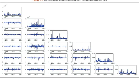
CCC for our series. Appendix B presents DCC (1,1) estimated parameters for our data sample. We note that all coefficients estimated for DCC (1,1) are statistically significant, but not all for the BEKK (2,1). Matrices A and B and diagonal coefficients of matrix C are all statistically significant. Other non-diagonal element of matrix C are not statistically significant. Estimated correlations from the two models are plotted in Appendix C.

As mentioned above, models are estimated using maximum

likelihood techniques which assume that residuals have normal

distributions. Thus, to check the fitted model robustness, we

check if residuals are white noise process. Figures in Appendix D

plots the standardized residuals from the estimated models, they

are calculated using the formula: X =H_{t t}

1

2. The first impression

we get from standardized residuals figures is that they are white noise.

We perform also Ljung-Box Q-test for residuals autocorrelation to examine if the standard residuals are random and independent

over time. Table 3 presents results of the Ljung-Box Q-test for residuals autocorrelation. Test statistics results reject the null

6 Burnham, K.P., Anderson, D.R. (2004), Multimodel inference:

Understanding AIC and BIC in model selection. Sociological Methods and

Research, 33, 261-304.

7 M = CC.

388

hypothesis that there is no autocorrelation. They are all greater than the critical. This rejects the conclusion we get from analyzing

standardized residuals plots.

Another examination of the adequacy of our model estimation in

capturing volatility and correlations dynamics is comparing the estimated volatility to the true volatility. While volatility is not

observable, we need to choose an approximation to it. The most common proxies of squared volatility are the squared returns and

realized volatility. Because realized volatility is based on intraday data that are not available for our assets, we will use in our

comparison squared returns as a proxy for volatility. We compute

volatilities for an equally weighted portfolio of ours assets, they are plotted in Figure 2. We notice that the estimated volatilities follow squared returns tendency.

4. MODELS COMPARISON

In addition of diagnostics done in the previous paragraph, we are going to use mean absolute error (MAE) of estimated and

Figure 1: Daily returns series plot

Table 1: Descriptive statistics of daily returns

Statistic IAM LESU CTM MNG SOND HOL

Mean (×10−17) −1214.7 35.12 12.48 16.51 −6.18 −29.56

Standard error 0.0298 0.0411 0.0503 0.0524 0.049 0.0428

Median 0.0088 −0.0091 0.0165 0.0327 −0.01 0.0345

Mode 0.0088 −0.0091 0.0165 0.0327 −0.01 0.0345

Standard deviation 1.564 2.1542 2.6378 2.7455 2.5669 2.2451

Sample variance 2.4462 4.6405 6.958 7.5377 6.5888 5.0403

Kurtosis 4.7566 3.4628 7.5508 5.7903 3.6587 4.8238

Skewness 0.3226 0.3325 −0.2358 0.1531 0.1256 0.3277

Minimum −8.0061 −9.7679 −24.8296 −13.6192 −12.4004 −10.9522

Maximum 10.6383 13.0937 16.5225 23.7386 13.4513 14.5111

JB statistic (×103) 2.6264 1.4168 6.5262 3.8328 1.5325 2.7013

Table 2: Model order selection

Model AIC BIC

BEKK

BEKK (1,1) −80251.31 −80056.00

BEKK (1,2) −80225.91 −79995.09

BEKK (2,1) −80448.27* −80217.44*

BEKK (2,2) −80294.76 −80028.42 DCC

DCC (1,1) −81175.41* −80968.26*

DCC (1,2) −81173.41 −80960.34

DCC (2,1) −81173.87 −80960.79

DCC (2,2) −81171.86 −80952.87

DCC: Dynamic conditional correlation, BEKK: Baba, Engle, Kraft and Kroner,

squared returns (volatility proxy) to compare models, the MAE

is computed as bellow:



N

k k

k=1 1 MAE

N

=

∑

Where, N is the number of observations, σˆ is empirical (squared

returns) and σ is estimated volatility at day k. Table 4 presents the MAE of each model:

MAE measures how close the estimated volatility from the empirical volatility. According to calculated values for both models, BEKK

model performs better than DCC. This result is in accordance with

the one we get when testing autocorrelation of standardized residuals

of each model. The Ljung-Box Q-test statistics of BEKK(2,1) is less than DCC(1,1) in almost all cases. This is an indication that

the part of autocorrelation explained by BEKK(2,1) model is more important than the one explained by DCC(1,1).

Another way to compare our models is checking the difference between the estimated volatilities. Figure 3 displays these

differences. The calculated differences are small with a mean equal to 3.78 × 10−6_{. The positive value of the mean indicates that}

volatility estimated by DCC model is higher than BEKK model9_.

To check if the two models well capture volatility clustering, we

perform ARCH LM test10_{. Appendix E Table presents results of}

this test before and after estimation. Table E1 presents test results

before the estimation. They show a high presence of volatility

clustering in our series. Table E1 contains results of ARCH LM test

of models residuals. Test statistics indicates that the null hypothesis of non-existence of ARCH effect (volatility clustering) in BEKK

9 Because we substructed BEKK estimated volatilies from DCC ones.

10 It assesses the null hypothesis that a series exhibits no conditional heteroscedasticity (ARCH effect), Engle, R. (1988), Autoregressive

conditional heteroscedasticity with estimates of the variance of United

Kingdom inflation. Econometrica, 96, 893-920.

Table 3: T-statistic Ljung-Box Q-test for of autocorrelation of standardized residuals

Model Lag IAM LESU CTM MNG SOND HOL Critical value

DCC (1,1) 5 71.38 82.97 135.48 36.33 34.26 73.74 11.07

DCC (1,1) 10 80.27 91.82 138.07 40.89 39.89 80.24 18.31

DCC (1,1) 15 82.72 95.84 139.12 42.81 45.87 85.13 25

DCC (1,1) 20 85.84 106.21 144.24 45.15 48.1 96.46 31.41

BEKK (2,1) 5 66.93 85.8 148.46 25.98 27.93 70.62 11.07

BEKK (2,1) 10 74.91 95.04 151.1 31.08 33.03 77.47 18.31

BEKK (2,1) 15 77.33 97.46 152.07 32.37 38.64 81.9 25

BEKK (2,1) 20 79.9 108.53 158.19 34.74 41.23 94.9 31.41

DCC: Dynamic conditional correlation, BEKK: Baba, Engle, Kraft and Kroner

Figure 2: Dynamic conditional correlation and Baba, Engle, Kraft and Kroner estimated volatility versus empirical volatility portfolio

Table 4: Models mean absolute errors model

MAE diagonal BEKK (×10−2) 2.7842

DCC (×10−2) 3.3567

DCC: Dynamic conditional correlation, BEKK: Baba, Engle, Kraft and Kroner,

390

models cannot be rejected for all lags. However, statistics of the

DCC(1,1) model indicate that it successfully captures volatility

clustering in our series as the null hypothesis is accepted for all them and for all lags.

4.1, Forecasting with BEKK and DCC Models\Label

After we estimated BEKK and DCC models, we can perform

volatility forecasting. Below the conditional covariance equation of the BEKK model:

( )

' ' ' '

t+1 t t t t

H = C C + A E ò ò Â + B ˆ ˆ ˆ ˆ ˆ H ˆB (12)

Forecast with DCC model is done through two steps procedure. As

stated in equation 8, the conditional covariance is written as below:

t+1 t+1 t+1 t+1

H =D Γ D (13)

The first step in the forecasting procedure with DCC model consists of predicting diagonal element of matrix D_t+1 using a

GARCH(1,1) process. The second step consists of estimating matrix Γ_t+1 using equation 9. Once both steps are completed, the conditional covariance of DCC model can be deduced.

We will perform forecast for our assets for the period from

21/10/2015 to 31/03/2016, the forecast is done ahead 1 day through

this period. Figure 4 plots the foretasted volatility results for our

equally weighted portfolio assets. The vertical dotted line in this figure separates estimation and forecast period. According to this figure, forecasted results show that they follow the same tendency

as the estimated ones, also, the forecasts with both models appear to be stable. Similarly to section 3.4, we use the MAE to evaluate

the quality of the forecasts. Table 5 presents the computed values

of MAE for our forecasted results with squared returns used as

volatility proxy. Computed MAE values show that DCC performs better than BEKK model: Computed MAE for DCC is lower than

BEKK model for all assets.

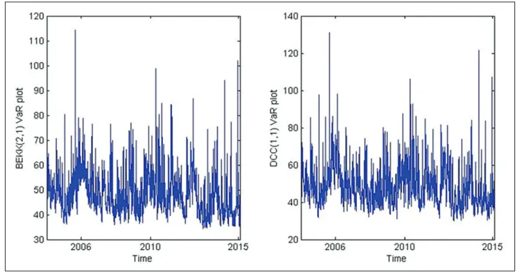
4.2. Application to VaR

VaR measures the potential loss in value of a portfolio over a

defined period at a given confidence interval. VaR is a capital

regularity requirement to financial institutions, it is considered as a measurement of risk they are exposed too. The VaR of a given portfolio is defined as below:

VaR( )=α α X′

∑

Where, α is the confidence interval, σ is the variance covariance matrix and X is a column vector of asset values.

Covariance matrices already estimated for both models will be used in equation 14, the obtained results will be used as a

performance measure to evaluate models DCC and BEKK in calculating VaR. The comparison is done through The dynamic quantile test introduced by Engle and Manganelli (2001)11_.

We define the hit variable:

11 Engle and Manganelli, (2001), Value-at-risk models in finance. Working

Paper 75, Working Paper Series, European Central Bank.

Figure 3: Difference between the estimated volatilities

Hit(α)=I_α (α)-α (15)

I_t(α) is the binary variable associated to past observations of VaR

violation at time t:

( )

( )

t 1, if r <VaR

I =

0, otherwise −

 α

α 

 (16)

VaR_t|t−1(α) is the conditional VaR

Each time VaR exceeds the asset value, the Hit variable takes the value of 1-α and α otherwise. From VaR definition, the Hit_t(α)

variable should be unpredictable based on its own lagged values or

any other variable, in particular, past VaR and assets returns. The

dynamic quantile test consists of testing the null hypothesis that

all coefficients and the intercept, of a regression of this variable

on its past values, VaR, and a set of other variables, are all null. In our study, we regress the hit variable on its past values (5 lags are taken), VaR, portfolio returns and squared portfolio returns.

Our regression equation is as below:

( )

k t k t t t t

k=1

Hit α γ= +

∑

Using an equally weighted portfolio for our stocks with a total

value of 1000 MAD, we calculate VaR over a 1 day horizon and at a 95% confidence level. Results are presented in Figure 5. Both

calculated VaRs have the same tendency, but DCC (1,1) model

tends to estimate relatively higher values in comparison with

BEKK (2,1) model. The dynamic quantile test regression results

are presented in Table E3. According to obtained P-values, two variables (the intercept and squared returns) are not statistically

significant, thus, the hypothesis of joint nullity of parameters of

the regression is rejected.

Engle and Manganelli deduced a simple test, under the null

hypothesis, The dynamic quantile test is equivalent to a conditional efficiency test. We denote by Ψ = (γ, β₁,…, β₅, θ, σ, λ) the vector of 2K+1 parameters and by Z the matrix of explanatory variables of equation 18. Wald statistic associated to conditional efficiency test, noted DQ_cc satisfies:



( ) (

)

' ' 2 cc Z ˆ

DQ = 2K+1

1-ψ 1-ψ χ

α α (18)

Test results reject the hypothesis of joint nullity of parameters of equation 18. The Wald statistics calculated are 10003.87 and 10005.76 for BEKK(2,1) and DCC(1,1) models respectively. These two values are highly greater than the critical value of chi-square distribution which is equal to 19.9190 at 9° of freedom and 1-α = 95% probability level. These results are in accordance with

regression results presented in Table E3. We conclude from the dynamic quantile test done that both models failed to adequately calculate VaR in the case of our selected stocks.

5. CONCLUSION

Volatility is a key element in risk and asset management. It is a measure of assets risk based on the variance of returns. Volatility

is not observable and then should be estimated. The most popular

methods in estimating volatility are historical volatility, implied

volatility and auto-regressive heterokedastic models, for example GARCH family models. The first model in GARCH family was introduced by Engle in 1982, the ARCH model, it was considered as a great invention in financial econometrics. Later on, many extensions of ARCH were developed, e.g., GARCH, EGARCH,

etc. GARCH family models are useful only in estimating volatility for Univariate dimension, they are enable to estimate volatility

Table 5: Models mean absolute errors for evaluating forecast

Model IAM LESU CTM MNG SOND HOL

DCC (×10−2) 1.005 2.5100 2.6426 1.6493 3.2112 4.7359

Diagonal BEKK (×10−2) 1.2548 2.5881 3.1159 1.7949 4.3989 5.2302

DCC: Dynamic conditional correlation, BEKK: Baba, Engle, Kraft and Kroner

392

and correlation when multiple assets are involved. Multivariate GARCH models were developed for this purpose.

The aim of this article was to examine correlation between stocks chosen from Casablanca stocks exchange markets using multivariate GARCH models. We selected six stocks that have the longest and continuous daily prices. Descriptive statistics of

our series showed that volatility is not constant over time, also, we noticed that our data suffers from volatility clustering, this was

confirmed by ARCH LM tests performed. We used in our study

the most widely used multivariate GARCH models, BEKK and

DCC. These two models have attracted a considerable interest in the financial econometric literature. Model order selection tests we performed showed that DCC(1,1) and BEKK(2,1) are the most suited to our series. The choice of DCC instead of CCC model

was based also on test of dynamic correlation which showed that correlation is not constant over time.

Estimated models comparison showed that BEKK (2,1) performs

better than DCC (1,1) in the case of our series. First the MAE in comparison to empirical volatility of BEKK is less than DCC, secondly, the Ljung-Box Q-test indicated that the part of volatility explained by BEKK is more important than DCC. However, we found out using ARCH LM test, that DCC captures well volatility clustering than do BEKK model. Another examination of estimated

models is comparing estimated volatility to the empirical one. We

used squared returns as a proxy for the empirical volatility. The computed values of the MAE showed that the fitting performance of BEKK is higher than DCC.

After we estimated BEKK and DCC for our series, we performed volatility forecasting. The forecasts with both models have the same tendency as estimated ones; also, they appear to be stable.

The comparison between forecasted and empirical volatility showed that DCC performs better than BEKK. The easy computation is another advantage of DCC model, we noticed

that it is less demanding in time than needs BEKK.

The estimated variance and covariance matrices using BEKK and DCC models were applied also to VaR calculation. VaR is one of the most popular tools used by financial institutions, it measures the maximum loss of a portfolio at a given confidence level and a time horizon. DCC model estimated a relatively high VaR values than BEKK, but with same tendency. The quality of

the estimation was tested using the dynamic quantile test of Engle

and Manganelli. This test results showed that both models failed

to adequately estimate VaR for our series.

REFERENCES

Alexander, C.O. (2001), A Primer on the Orthogonal GARCH Model.

ISMA Centre, University of Reading, Working Paper.

Black, F. (1976), Studies of stock price volatility changes. In: Proceedings of the 1976 Meetings of the American Statistical Association,

Business and Economics Statistics Section. p177-181.

Bollerslev, T. (1986), Generalized autoregressive conditional heteroskedasticity. Journal of Econometrics, 31(3), 307-327. Bollerslev, T. (1990), Modelling the coherence in short-run nominal

exchange rates: A multivariate generalized ARCH model. The Review of Economics and Statistics, 72(3), 498-505.

Bollerslev, T., Chou, R.Y., Kroner, K.F. (1992), ARCH modeling in finance. Journal of Econometrics, 52(1), 5-59.

Bollerslev, T., Engle, R.F., Wooldridge, J.M. (1988), A capital asset

pricing model with time-varying covariances. Journal of Political

Economy, 96(1), 116-131.

Christie, A.A. (1982), The stochastic behavior of common stock variances:

Value, leverage and interest rate effects. Journal of Financial

Economics, 10(4), 407-432.

Ding, Z., Granger, C.W.J. (1996), Modeling volatility persistence of

speculative returns: A new approach. Journal of Econometrics, 73(1), 185-215.

Ding, Z., Granger, C.W.J., Engle, R.F. (1993), A long memory property

of stock market returns and a new model. Journal of Empirical

Finance, 1(1), 83-106.

Engle, R. (2002), Dynamic conditional correlation: A simple

class of multivariate generalized autoregressive conditional heteroscedasticity models. Journal of Business and Economic

Statistics, 20(3), 339-350.

Engle, R., Kelly, B. (2012), Dynamic equicorrelation. Journal of Business and Economic Statistics, 30(2), 212-228.

Engle, R.F. (1982), Autoregressive conditional heteroscedasticity with estimates of the variance of United Kingdom inflation. Econometrica, 50(4), 987-1007.

Engle, R.F., Kroner, K.F. (1995), Multivariate simultaneous generalized arch. Econometric Theory, 11(1), 122-150.

Engle, R.F., Ng, V.K., Rothschild, M. (1990), Asset pricing with a

factor-arch covariance structure. Journal of Econometrics, 45(1), 213-237.

Engle, R.F., Sheppard, K. (2001), Theoretical and Empirical Properties of Dynamic Conditional Correlation Multivariate Garch. 8554, October, 2001.

Jobson, J.D., Korkie, B. (1989), A performance interpretation of multivariate tests of asset set intersection, spanning, and mean-variance efficiency. Journal of Financial and Quantitative Analysis, 24(2), 185-204. Manganelli, S., Engle, R.F. (2001), Value at Risk Models in Finance.

European Central Bank, (Working Paper No. 75), August, 2001. Merton, R.C. (1972), An analytic derivation of the efficient portfolio frontier.

The Journal of Financial and Quantitative Analysis, 7(4), 1851-1872. Merton, R.C. (1980), On estimating the expected return on the market.

Journal of Financial Economics, 8(4), 323-361.

Nelson, D.B. (1991), Conditional heteroscedasticity in asset returns: A new approach. Econometrica, 59(2), 347-370.

Officer, RR. (1973), The variability of the market factor of the New York stock exchange. The Journal of Business, 46(3), 434-453.

Pindyck, R. (1984), Risk, inflation, and the stock market. American

Economic Review, 74(3), 335-351.

Roll, R. (1977), A critique of the asset pricing theory's tests part I: On

past and potential testability of the theory. Journal of Financial

APPENDICES

Appendix A: BEKK (2,1) coefficients estimation

Coefficient Estimation Standard error t-statistic

M (1,1) 0.000203 0.0000124 16.413 M (1,2) 0.00000219 0.00000303 0.72333

M (1,3) 0.00000138 0.00000263 0.524411

M (1,4) −0.00000145 0.00000373 −0.389404

M (1,5) −0.00000748 0.00000556 −1.346126

M (1,6) 0.000000726 0.00000334 0.217124

M (2,2) 0.0000154 0.00000168 9.147694

M (2,3) −0.000000529 0.000000896 −0.590486

M (2,4) −0.00000107 0.000000985 −1.089826

M (2,5) 0.00000389 0.00000288 1.347909

M (2,6) −0.0000000321 0.000000701 −0.045746

M (3,3) 0.0000288 0.00000244 11.81638 M (3,4) 0.00000112 0.00000106 1.057964

M (3,5) −0.000000104 0.00000253 −0.041084

M (3,6) −0.000000372 0.000000732 −0.508196

M (4,4) 0.0000304 0.00000287 10.60451

M (4,5) 0.00000131 0.00000322 0.406006

M (4,6) −0.000000539 0.000000879 −0.613408

M (5,5) 0.000161 0.0000146 10.98759

M (5,6) 0.00000451 0.00000298 1.512518 M (6,6) 0.00000357 0.000000444 8.037292

A1 (1,1) 0.353479 0.020463 17.27423 A1 (2,2) 0.295759 0.014473 20.4352

A1 (3,3) 0.278994 0.014584 19.1305

A1 (4,4) 0.327969 0.012393 26.46482 A1 (5,5) 0.482548 0.015469 31.19477

A1 (6,6) 0.017377 0.015566 1.116374 A2 (1,1) −0.455349 0.023959 −19.00575

A2 (2,2) −0.2132 0.021748 −9.803076

A2 (3,3) −0.100728 0.029604 −3.402446

A2 (4,4) 0.132033 0.027061 4.879112

A2 (5,5) 0.281524 0.033555 8.390009

A2 (6,6) −0.155057 0.005977 −25.9433

B1 (1,1) 0.646748 0.019445 33.26066

B1 (2,2) 0.920644 0.005184 177.5853 B1 (3,3) 0.892339 0.008073 110.528

B1 (4,4) 0.90744820 0.005967 152.0782

B1 (5,5) 0.71512 0.021343 33.50623

B1 (6,6) 0.984682 0.001094 900.3076

BEKK: Baba, Engle, Kraft and Kroner

Appendix B: DCC (1,1) coefficients estimation

Parameter Estimation Standard error t-value

ω₁ 135.28013 86.58288 1.562435091

α₁ 0.2712445 0.3367281 0.805529743

β₁ 0.762976403 0.007835544 97.37376282

ω₂ 165.1068612 0.1495558 1103.981666

α₂ 0.329009 0.1326704 2.479897551

β₂ 0.77881184 0.02112435 36.86796706

ω₃ 0.6372866 0.0610729 10.43485081

α₃ 0.41494041 0.03610632 11.49218226

β₃ 0.757185753 0.007019868 107.8632466

ω₄ 75.39039 108.76261 0.69316459

α₄ 0.1070037 162.6292249 0.000657961

β₄ 0.78191449 0.01259818 62.0656706

ω₅ 0.00178703 0.14218614 0.012568243

α₅ 0.02998864 0.28244741 0.106174243

β₅ 0.97726531 0.04096206 23.85781648

ω₆ 0.001356091 0.069170771 0.019604972

α₆ 0.173388 0.4464916 0.388334293

β₆ 0.88502061 0.02477999 35.71513185

DCCα 0.02011386 0.000254597 79.00283036

DCCβ 0.03955214 0.32286853 0.122502308

394

Appendix C

Figure C1: Diagonal Baba, Engle, Kraft and Kroner model estimated correlations plot

Figure D1: Baba, Engle, Kraft and Kroner model standardized residuals plot Appendix D

396

Appendix E

Table E1: ARCH LM test for daily returns

Series IAM LESU CTM MNG SOND HOL

P value 0 0 0 0 0 0

Test statistic 70.4189 132.6917 64.1082 89.5894 72.7168 113.9469

Critical value 3.8415 3.8415 3.8415 3.8415 3.8415 3.8415

ARCH: Autoregressive conditional heteroskedasticity

Table E2: ARCH LM tests for standardized residuals

Model Lag Variable IAM LESU CTM MNG SOND HOL

DCC (1,1) 1 P value 0.5903 0.2470 0.4319 0.8208 0.4163 0.3343

Test statistic 0.2899 1.3399 0.6177 0.0513 0.6606 0.9323

Critical value 3.8415 3.8415 3.8415 3.8415 3.8415 3.8415

5 P value 0.5074 0.4419 0.7847 0.7379 0.2634 0.3167

Test statistic 4.2978 4.7913 2.4455 2.7539 6.4668 5.8941

Critical value 11.0705 11.0705 11.0705 11.0705 11.0705 11.0705

10 P value 0.4450 0.6387 0.8964 0.9044 0.4341 0.3057

Test statistic 9.9485 7.8987 4.9213 4.7949 10.0736 11.6994

Critical value 18.3070 18.3070 18.3070 18.3070 18.3070 18.3070

20 P-value 0.0924 0.0248 0.9980 0.6261 0.1185 0.1288

Test statistic 28.7685 34.2082 6.4938 17.4116 27.6275 27.2355

Critical value 31.4104 31.4104 31.4104 31.4104 31.4104 31.4104

BEKK (2,1) 1 P value 0.0103 0 0.3192 0.0201 0 0

Test statistic 6.5880 74.6317 0.9921 5.4027 20.4242 33.0170

Critical value 3.8415 3.8415 3.8415 3.8415 3.8415 3.8415

5 P value 0.0483 0.0000 0.9304 0.0993 0.0000 0.0000

Test statistic 11.1624 76.6855 1.3435 9.2558 33.8767 35.7401

Critical value 11.0705 11.0705 11.0705 11.0705 11.0705 11.0705

10 P value 0.0994 0.0000 0.9880 0.1226 0.0001 0.0000

Test statistic 16.0075 80.6279 2.6777 15.2671 36.0209 40.4832

Critical value 18.3070 18.3070 18.3070 18.3070 18.3070 18.3070

20 P value 0.0994 0.0000 0.9880 0.1226 0.0001 0.0000

Test statistic 16.0075 80.6279 2.6777 15.2671 36.0209 40.4832

Critical value 18.3070 18.3070 18.3070 18.3070 18.3070 18.3070 ARCH: Autoregressive conditional heteroskedasticity, DCC: Dynamic conditional correlation, BEKK: Baba, Engle, Kraft and Kroner

Table E3: Hit regression results

BEKK (2.1)

Variable Estimate Standard error t-Stat P-value

(Intercept) 0.515864396 0.038631123 13.35359553 1.89×10-39

H itt−1 −0.000961118 0.012400926 −0.077503762 0.93822847

H itt−2 −0.013410133 0.012349631 −1.085873133 0.277630857

H itt−3 0.00592022 0.012355105 0.479171987 0.631854604

H itt−4 −0.018955998 0.012358024 −1.533902056 0.125169454

H itt−5 0.010050019 0.012298799 0.817154508 0.413911337

VaRt −0.000582008 0.000707428 −0.822710689 0.410744284

rt −4.9×10-9 3.78×10-9 −1.295739961 0.19517447

rt2 −0.000396445 0.00000637 −62.23433128 0

DCC (1.1)

(Intercept) 0.501959029 0.03302687 15.19850449 3.83×10-50

H itt−1 −0.000799852 0.012404143 −0.064482643 0.948590642

H itt−2 −0.013250749 0.01234836 −1.073077657 0.283330979

H itt−3 0.006080367 0.012354503 0.492157991 0.622647174

H itt−4 −0.018782073 0.012356715 −1.519989192 0.128629324

H itt−5 0.01024675 0.012296703 0.833292402 0.40475263

VaRt −0.000303418 0.000583455 −0.520037083 0.603079833

rt −0.00000000497 0.00000000381 −1.304049237 0.192326573

rt2 −0.000396501 0.00000637 −62.23204228 0