Prediction of the Moving Direction of Google Inc.
Stock Price Using Support Vector Classification and
Regression
Liu Pan
Department of Business English, Gannan Normal University
Economic & Technological Development Zone, Ganzhou 341000, China
E-mail: [email protected]
Xuan Liu(Corresponding author)
Department of Electrical and Computer Engineering, Johns Hopkins University
3400 N. Charles St, Baltimore, MD, USA.
Tel: 1-90-6487-1634 E-mail: [email protected]
Received: April 16, 2014 Accepted: May 18, 2014 Published: June 1, 2014
doi:10.5296/ajfa.v6i1.5485 URL: http://dx.doi.org/10.5296/ajfa.v6i1.5485
Abstract
Keywords: Financial forecasting, Stock price prediction, Trend prediction, Technical
1. Introduction
Analysis of stock market, including the stock price forecasting, has long been an intriguing topic for both investigators and researchers. Fundamental analysis and technical analysis are the two main stock analysis strategies used to forecast the future stock price movements (Murphy, 1999; Turner, 2007). Fundamental analysis attempts to predict the price of a particular stock by studying the company fundamentals such as revenues, annual growth rates, and potential competitors (Murphy, 1999). Technical analysis, on the other hand, is solely based on the study of stock market's historical data or pattern, including price, volume action and technical indicators (Turner, 2007). Both approaches have their own Pros and Cons. Generally, fundamental analysis is favored for longer time frames, while technical analysis is considered as a better style for short-term trading.
Forecasting the short-term trend of a stock market is still a big challenging task nowadays. This is because that stock market is noisy, chaotic, nonparametric and non-linear in nature, and many external entities like politics, human psychology/behavior, liquid money and related news influence the direction of the stock market (Abu-Mostafa and Atiya, 1996). Recently, a lot of interesting work has been carrying on in the area of applying machine learning algorithms, including support vector machine (SVM), for analyzing price patterns and predicting stock prices and index changes (Yang et al., 2002; Grosan and Abraham, 2006; Chen et al., 2006; Sapankevych and Sankar, 2009; Kao et al., 2013; Kazem et al., 2013; Zhi-gang et al., 2013). The advantage of SVM is that it is able to reach the global optimum and is resistant to the undertraining or overtraining problems (Yoo et al., 2005; Chen et al., 2006; Sapankevych and Sankar, 2009). This machine learning method has been successfully used for stock return predictions in several financial areas (Yang et al., 2002; Chen et al., 2006; Sapankevych and Sankar, 2009; Kao et al., 2013; Kazem et al., 2013).
Parameters of stock markets, including open/close prices, daily-high/low prices and trading volumes, were frequently used in previous studies to forecast the stock market (Lildholdt, 2002; Fiess and MacDonald, 2002; Corwin and Schultz, 2012; Fuertes and Olmo, 2013). Considering that the moving trends of these parameters may have certain inertia within short-term period, we hypothesized that the moving direction of these parameters would be better than the original parameters themselves for predicting the short-term stock price. To test this hypothesis, in this study we explored the potential application of the moving trends of these stock parameters to forecast the movement direction of stock price of Google Inc. by using support vector classification (SVC) and support vector regression (SVR), two main SVM application forms.
The remaining sections of this report are organized as following: section 2 provides a brief overview of the SVM algorithms; Section 3 describes the experiment design; Section 4 reports and discusses the experiment results; Section 5 summarizes the whole report.
2. Methodology
2.1 The basic ideas of SVC and SVR
capacity control obtained by acting on the margin or on number of support vectors (Vapnik, 1995). According to the purposes,SVMs can be divided into SVC, SVR, and ranking SVM. SVC performs classification by finding the hyperplane that maximizes the margin between the two classes in high- or infinite-dimensional space. SVR is extended from SVM and performs regression in the high-dimension feature space using insensitive loss. Both SVC and SVR are widely used in various areas and continue to be two of the most successful machine learning algorithms. An overview of the basic ideas of SVC and SVR was described in detail in reference (Yoo et al., 2005). Briefly, for a two-class classification problem, we can assume that we have a set of input data points xi ∈ Rd(i = 1,2,...,N) along with each point’s classification yi, where yi can take on one of two possible values: -1 or 1. The linear support vector machine is defined as the following optimization problem:
min w
1 2 w
T
·w + C
l
i=1 ξi
s.t. yi(wt ·xi + b) ≥ 1 −ξ, ξi ≥ 0 i = 1...l
where ξi is the error for a given training point xi, w is the margin, b is the offset for the hyperplane, and C is a constant representing the emphasis that is to be placed on minimizing the error. The solution to this problem results in the following classifier for the prediction of f(x) in the new sample x:
f(x) = sign(
l
i=1
yiαi ·K(x,xi)+b)
where αI is the parameter coefficient, and K(x,xi) is kernel function.
For SVR, it is formulated as minimization of the following functional:
min w, b
1 2 w
T
·w + C
l
i=1
(ξi + ξi*)
s.t.
yi − (wT ·xi + b) ≤ε + ξi
(wT · xi + b) − yi ≤ ε + ξi*
ξi,ξi* ≥ 0,
i=1..l
Where ε is the parameter epsilon and the couple (xi, yi) the training Set. Slack variables ξ and
f(x) ≡
l
i=1
(αI − αi*)·K(x, xi) + b
2.2 Kernel and optimization of kernel parameters
Epsilon-SVR in LIBSVM package, which is developed by Chang et al (2011) and is currently one of the most widely used SVM, was employed for stock price prediction in this study. LIBSVM supports four basic kernel functions (Hsu et al., 2005; Chang and Lin, 2011):
(1) Linear Kernel: K(x, y) = x·y
(2) Polynomial Kernel: K(x,y) = (γ·x·y + coef0)degree
(2) Radial Basis function (RBF) Kernel: K(x,y) = exp (-γ·||x - y||2) (3) Sigmoid Kernel: K(x,y) = tanh (γ ·x·y +coef0)
We chose RBF Kernel in our study because of the following factors: 1) RBF kernel has fewer numerical difficulties and can handle the nonlinear models (Hsu et al., 2005); 2) The linear kernel can be regard as a special case of RBF Kernel; 3) The polynomial kernel has more hyperparameters than the RBF kernel; 4) The sigmoid kernel behaves like RBF for certain parameters (Hsu et al., 2005).
TheSVMperformancedepends on a good setting of two parameters C and γ (Hsu et al., 2005; Chang and Lin, 2011). Basing on 3-fold cross-validationerror, we obtained the best valuesof parameters C and γ for SVC and SVR using grid search method.
3. Experiment Design
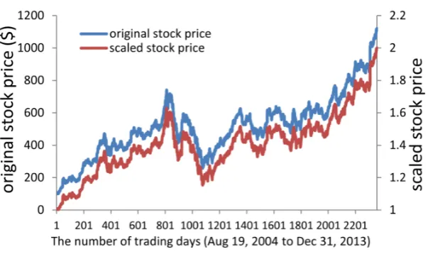
Figure 1. The overall moving trend of original (left y-axis) and scaled (right y-axis) close price for Google Inc. for the year of 2004 to 2013
To examine within which time period the moving trend will be better for prediction of the stock direction, in this study we analyzed the prediction accuracy of the moving trends of GOOG transaction data within 4 different time periods, including periods of 5, 15, 30 and 45 trading days, respectively. The SVM classifiers generated basing on the 4 moving trends are named correspondingly as classifiers 1, 2, 3 and 4, respectively. The moving trend of the transaction data within a time period is defined as the slope (value b) in the regression formula Y= a + bX that is produced by simple linear regression analysis, in which X is the number of trading day (from 1 to 5 for classifier 1, 1 to 15 for classifier 2, 1 to 30 for classifier 3 and 1 to 45 for classifier 4), and Y is the corresponding data (open price, high price, low price, close price or volume) at the corresponding trading date. The obtained slopes of the open prices, high prices, low prices, close prices and volumes of GOOG within 5 (classifier 1), 15 (classifier 2), 30 (classifier 3) or 45 (classifier 4) training days were then used as five input features for SVM to predict the slopes of close price of GOOG in the next 5th, 15th, 30th or 45th days, respectively. The predicted slope of GOOG close price >0 represents the stock price rose up during that period, while slope <0 means price falling down.
To check the prediction accuracy, the predicted results were compared with the actual data (called indicator). The slope values of the close price of GOOG were directly used as indicators in SVR analysis. In SVC analysis, a Boolean value (1 or -1) that was transformed from the slope values of the close price was used as indicators. Boolean value ‘1’ means the corresponding slope value >0, while ‘-1’ means the corresponding slope <0.
to 2 using Mapminmax function of Matlab before applying SVM analysis. Figure 1 shows that scaled close prices have the exactly same pattern as that of the original close prices.
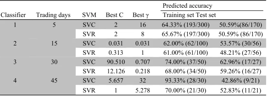
The best values for parameter C and γ that were obtained by grid search method for each of the SVR perdition classifier are shown in Table 1.
4. Results and Discussions
4.1 Prediction of moving direction of GOOG price using SVC
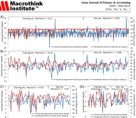
SVC analysis gave out a probability value ranging from 0 to 1 for each instance (e.g. moving direction in one trading period). The probability value closing to 1 means that the chance for GOOG stock price rising up is very high, closing to 0 means the great chance of price falling down, while close to 0.5 represents the chance of price rising-up is similar to that of falling down. Figure 2 shows the correlation between the predicted probability values and actual moving trend (slope) across all the instances analyzed. Among the 4 classifiers, the predicted pattern in classifier 3 (slopes within 30 trading days) is the most closest to the actual moving trend and has the highest Pearson’s correlation coefficients (Pearson’s r) in both training and test datasets.
Table 1. SVM parameters and prediction accuracies for different classifiers tested
Classifier Trading days SVM Best C Best γ
Predicted accuracy Training set Test set
1 5 SVC 2 16 64.33% (193/300) 50.59%(86/170)
SVR 2 8 65.67% (197/300) 50.59% (86/170)
2 15 SVC 0.031 0.031 62.00% (62/100) 53.57% (30/56)
SVR 0.313 1 61.00% (61/100) 48.21% (27/56)
3 30 SVC 90.510 0.707 74.00% (37/50) 62.96% (17/27)
SVR 12.126 0.218 68.00% (34/50) 59.26% (16/27)
4 45 SVC 5.657 32 93.33% (28/30) 42.86% (9/21)
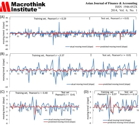
Figure 2. The correlation between the predicted possibility values and actual moving trend (slope) across all the instances (moving direction in one trading period) analyzed by SVC. (A)
Classifier 1 (5d). (B) Classifier 2 (15d). (C) Classifier 3 (30d). (D) Classifier 4 (45d).
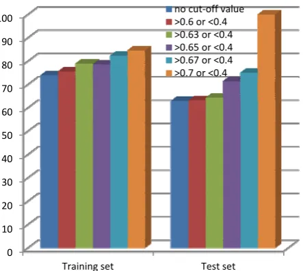
Figure 3. The Prediction accuracies when using more stringent cut-off values for the SVC classifier 3 to make classification
4.2 Prediction of moving direction of GOOG price using SVR
SVR analysis gave out a predicted slope value for each instance. Figure 4 shows the correlation between the predicted and actual slope values across all the instances analyzed. Like the SVC results, the predicted slope pattern in classifier 3 is the most closing to the actual pattern and has the highest Pearson’s r in both the training and test datasets. While for the other 3 classifiers, the patterns between predicted and actual slopes are similar only in the training dataset.
If we only consider whether the predicted moving direction by SVR is the same as the actual one (e.g., the predicted and actual slopes are both >0 or <0), we can also obtain the prediction accuracy data through the SVR analysis (Table 1). Similar to the SVC analysis, classifier 3 achieved the highest accuracy (59.26%) while the other 3 classifiers showed accuracies around 50% for the test dataset.
We also tried to use more stringent cut-off values for the classification basing on the SVR results. Again, higher prediction accuracies were achieved for the classifiers 2 and 3, especially the latter (Table 3). For example, the accuracy is 100% for the test dataset if instances with predicted slope values > 1 are classified into the price-rising up group and instances with values < -0.2 into the price-falling down group for classifier 3 (Figure 5).
0 10 20 30 40 50 60 70 80 90 100
Figure 4. The correlation between the predicted and actual slope values across all the instances analyzed by SVR. (A) Classifier 1. (B) Classifier 2. (C) Classifier 3. (D) Classifier
4
Figure 5. The prediction accuracies when using more stringent cut-off values for the classifier 3 basing on the SVR results
0 10 20 30 40 50 60 70 80 90 100
4.3 Prediction of moving direction of GOOG price using SVC and SVR combination
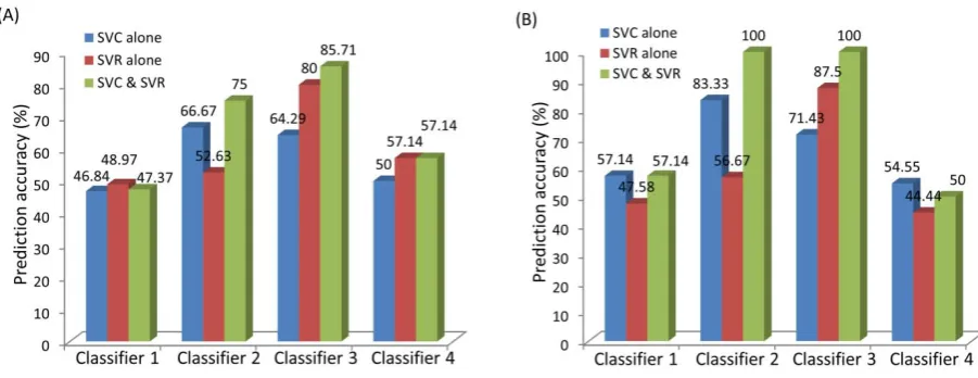
Figure 6 shows that combined use of SVC and SVR improves the prediction accuracy of the moving trend of GOOG stock price for classifier 2 and 3, especially the latter. We tested combinations at two levels. One is the combination of the classification results obtained when using the second cut-off value for SVC and SVR. The other one is the combination of the results when using the third cut-off vale for SVC and SVR. The principle for this combination is that only the instance classified into same group basing on SVC and SVR results are counted, and then the prediction accuracy are calculated basing on the percentage of instances being correctly classified by SVC and SVR.
Figure 6. Combined using SVC and SVR improves the prediction accuracy for the moving trend of GOOG stock price. Columns represent the prediction accuracy for the test sets. (A) Combined analysis of the prediction results that were obtained using the second cut-off vale for SVC (>0.61 or <0.4) and SVR (>0.4 or <-0.4). (B) Combined results that were obtained
using the third cut-off vale for SVC (>0.62 or <0.4) and SVR (>0.6 or <-0.6).
5. Summary
of stock transaction data within a certain time period have good inertia and are thus useful for forecasting the moving direction of stock price.
References
Abu-Mostafa, Y. S., & Atiya, A. F. (1996). Introduction to financial forecasting. Applied
Intelligence,6, 205-213. http://dx.doi.org/10.1007/BF00126626
Chang, C. and Lin C. (2011). LIBSVM : a library for support vector machines. ACM
Transactions on Intelligent Systems and Technology, 2, 1-27.
http://dx.doi.org/10.1145/1961189.1961199
Chen, Wun Hua, Shih, Jen Ying, & Wu, Soushan. (2006). Comparison of support-vector machines and back propagation neural networks in forecasting the six major Asian stock markets. International Journal of Electronic Finance, 1, 49-67. http://dx.doi.org/10.1504/IJEF.2006.008837
Corwin, Shane A. and Schultz, Paul. (2012). A Simple Way to Estimate Bid-Ask Spreads from Daily High and Low Prices. The Journal of Finance, 67, 719-760. http://dx.doi.org/10.1111/j.1540-6261.2012.01729.x
Fiess, Norbert M., & MacDonald, Ronald. (2002). Towards the fundamentals of technical analysis: analysing the information content of High, Low and Close prices. Economic
Modelling, 19, 353-374.
http://www.sciencedirect.com/science/article/pii/S0264999301000670
Fuertes, Ana Maria, & Olmo, Jose. (2013). Optimally harnessing inter-day and intra-day information for daily value-at-risk prediction. International Journal of Forecasting,29, 28-42. http://dx.doi.org/10.2139/ssrn.1924237
Grosan C, & Abraham A. (2006) Stock Market Modeling Using Genetic Programming Ensembles. In: Nedjah N, Mourelle L, Abraham A, editors. Genetic Systems Programming. 13 ed., 131-46. Springer Berlin Heidelberg. http://dx.doi.org/10.1007/3-540-32498-4_6
Hsu C-W, Chang C-C, & Lin C-J. (2005) A Practical Guide to Support Vector Classication. http://www.csie.ntu.edu.tw/~cjlin.
Kao, Ling Jing, Chiu, Chih Chou, Lu, Chi Jie, & Yang, Jung Li. (2013). Integration of nonlinear independent component analysis and support vector regression for stock price forecasting. Neurocomputing,99, 534-542. http://dx.doi.org/10.1016/j.neucom.2012.06.037
Kazem, Ahmad, Sharifi, Ebrahim, Hussain, Farookh Khadeer, Saberi, Morteza, & Hussain, Omar Khadeer. (2013). Support vector regression with chaos-based firefly algorithm for stock market price forecasting. Applied Soft Computing, 13, 947-958. http://dx.doi.org/10.1016/j.asoc.2012.09.024
Lildholdt P. (2002). Estimation of GARCH models based on open, close, high, and low prices. CAF, Centre for Analytical Finance.
Murphy J. J. (1999). Technical analysis of the financial markets: a comprehensive guide to
trading methods and applications, 2. Prentice Hall Press.
Turner T. (2007). A Beginner's Guide to Day Trading Online. Adams Media, 2nd edition. Vapnik V. (1995). The Nature of Statistical Learning Theory. Springer, N.Y., ISBN 0-387-94559-8.
Yang H, Chan L, & King I. (2002). Support Vector Machine Regression for Volatile Stock Market Prediction. In: Yin H, Allinson N, Freeman R, Keane J, Hubbard S, editors.
Intelligent Data Engineering and Automated Learning-IDEAL 2002. 2412 ed. Springer Berlin
Heidelberg; p. 391-6.
Yoo PD, Kim MH, & Jan T. (2005). Proceedings of the 2005 International Conference on Computational Intelligence for Modelling, Control and Automation, and International Conference on Intelligent Agents, Web Technologies and Internet Commerce (CIMCA-IAWTIC'05).
Zhi-gang, Wang, Chi-she, Wang, Qing-xia, Ma, & Yong, Hu. (2013). The securities market month K line forecast based on SVC. Information Science and Management Engineering