Activity modes selection for project crashing through deterministic simulation

JIEM, 2011 – 4(4):610-623 – Online ISSN: 2013-0953 – Print ISSN: 2013-8423 http://dx.doi.org/10.3926/jiem.224

Activity modes selection for project crashing through

deterministic simulation

Ashok Mohanty

, Jibitesh Mishra

, Biswajit Satpathy

1

College of Engineering and Technology Bhubaneswar,

Sambalpur University (INDIA)

[email protected]; [email protected]; [email protected]

Received July 2010 Accepted November 2011

Abstract:

Purpose:

The time-cost trade-off problem addressed by CPM-based analytical

approaches, assume unlimited resources and the existence of a continuous

time-cost function. However, given the discrete nature of most resources, the activities

can often be crashed only stepwise. Activity crashing for discrete time-cost

function is also known as the activity modes selection problem in the project

management. This problem is known to be NP-hard. Sophisticated optimization

techniques such as Dynamic Programming, Integer Programming, Genetic

Algorithm and Ant Colony Optimization have been used for finding efficient

solution to activity modes selection problem. The paper presents a simple method

that can provide efficient solution to activity modes selection problem for project

crashing.

Design/methodology/approach:

Simulation based method implemented on

electronic spreadsheet to determine activity modes for project crashing. The

method is illustrated with the help of an example.

Research limitations/implications:

The simulation based crashing method

presented in this paper is developed to return satisfactory solutions but not

necessarily an optimal solution.

Practical implications:

The use of spreadsheets for solving the Management

Science and Operations Research problems make the techniques more accessible

to practitioners. Spreadsheets provide a natural interface for model building, are

easy to use in terms of inputs, solutions and report generation, and allow users to

perform what-if analysis.

Originality/value: The paper presents the application of simulation implemented

on a spreadsheet to determine efficient solution to discrete time cost tradeoff

problem.

Keywords: project management, activity crashing, CPM, simulation, optimization

1 Introduction

Completing the project within time and cost limits are two important objectives of project management. The cost of a project is not due solely to the direct costs associated with individual activities in the project. Normally, there are indirect expenses as well that include overhead items such as managerial services, indirect supplies, equipment rentals, allocation of fixed expenses, interest on locked up capital already spent on project and so forth. These expenses are directly affected by the length of the project. In addition, the projects are generally bound by some contract, which specifies significant penalties for delay in completion of project beyond a given due date (deadline). So it is necessary to expedite the work for its timely completion.

Since minimizing time and cost are both preferred by the project manager, the project expediting process can be transferred to the typical time-cost trade-off analysis (Sunde & Lichtenberg, 1995). Time-cost trade-off means that we can shorten (i.e. crash) the duration of an activity by using additional resources/ cost (Wiest & Levy, 1977; Yau & Ritchie, 1990).

approaches we assume existence of unlimited resources and a continuous time-cost function. The analytical method involves lot of computation work and is difficult to apply even to a medium sized project consisting of hundreds of activities (Panagiotakopouols, 1977). Further, in many cases the time-cost function is non-linear. This makes the problem still more complicated to be solved by analytical methods. Due to discrete nature of most resources, in many practical situations time-cost function is not continuous and the activities can only be crashed stepwise. De et al. (1997) have shown strong NP-hardness of this problem. Due to unlikely existence of any polynomial algorithm to solve this problem optimally, the efforts have turned to finding the approximation and heuristics methods (Skutella, 1998; Tareghian, 2006; Rahimi, 2008).

There are several approximate algorithms that stipulate decision parameters and rules for selecting activities for crashing. These methods may give near optimal results. But these do not guarantee optimality and are proven to be problem dependent (Burns et al., 1996). Several sophisticated optimization and soft-computing techniques such as Dynamic Programming, Integer Programming, Genetic Algorithm, Ant Colony Optimization have been used to find efficient solution to activity modes selection problem.

During last one decade there has been a tremendous growth in the use of spreadsheets for solving various MS/OR problems both by the practitioners and the academic community. Seal (2001) has presented a review of MS/OR models in spreadsheets. He has also developed a generalized PERT/CPM implementation in a spreadsheet. The use of spreadsheets for solving the Management Science and Operations Research problems make the techniques more accessible to practitioners. Spreadsheets provide a natural interface for model building, are easy to use in terms of inputs, solutions and report generation, and allow users to perform what-if analysis.

This paper shows that a simple approach based on heuristic and deterministic simulation can give good result comparable to these sophisticated methods. The method is implemented on spreadsheet and is illustrated with the help of a simple example of project consisting of activities having discrete time-cost relationship.

2 Approaches for activity crashing

 Approach 1: Identify various assignable parameters that affect the solution and determine their relationship with solution output. Find a solution based on assignable parameters. Due to NP-hardness of this problem, the solution obtained in this approach may be fair but not likely to be an efficient solution.

 Approach 2: Evaluate all possible (generate very large number of random) solutions using deterministic simulation and choose the best one. However due to constraint on computing power and time, it may not always be possible to evaluate all possible solutions.

 Approach 3: Evaluate comparatively much lesser number of solutions around the space where there is more likelihood of finding the efficient (optimal) solution and select the best one.

3 Solution through limited search

Most of the soft-computing algorithms are based on this third approach for finding the efficient (optimal) solution. For example, in Genetic Algorithm (GA), we usually find few solutions at random and pick the best two solutions. Then by crossover and mutation, we determine more solutions (off-springs), which are nearer to the parent solutions. From these the best ones are selected to generate more off-springs. Here crossover ensures similarity with parent solutions and mutation causes some random variations in off-springs. So instead of evaluating all possible solutions, we evaluate a much lesser number to arrive at an efficient solution.

4 Selection of parameters for activity crashing

Let a project comprises of number of interrelated activities having discrete time-cost relationship. In a simple form, each activity of project can be executed either in normal mode or in expedited (crashed) mode. The attributes of project activities can also be represented by arrays as given below.

NDi = Normal duration of activity “i”

CDi = Crashed duration of activity “i”

CCi = Cost of executing activity “i” in crashed/ expedited mode

EMi = Execution mode of activity “i”. EMi is 0 or 1 depending upon if activity “i” is executed in Normal mode or Expedited mode.

The activities can be selected for execution in expedited (crashed) mode based on number of known parameters, such as criticality of activity, extra cost to be incurred and consequent reduction in activity duration due to executing the activity in expediting mode, etc. We may combine a number of such parameters to devise a single index, which may indicate the suitability of the activity for execution in expedited mode. We may refer this index as Activity Index for Expediting (AIE). Let AIE for an activity „i‟ is denoted by Mi. Some possible parameters to determine AIE are given below.

 Cost incurred for executing an activity in expedited (crashed) mode. If cost is more, the activity is less suitable for being executed in expediting mode. So Activity Index for Expediting Mi, for activity “i” is inversely proportional

to crashing cost, i.e.

M



(

1

/

CC

)

activity “i” is directly proportional to effectiveness of activity crashing.i.e.

Miα CEi

 Delay in execution of an activity affects its succeeding activities. So number of immediate succeeding activities of an activity may be considered as another indicator of its criticality. Two activities may have same float but the one that has more succeeding activity may be considered as more critical. So Activity Index for Expediting Mi, for activity “i” is directly proportional to number of immediate succeeding activities, SAi. i.e. MiαSAi.

So Mi may be determined as under.

i i i i

CC

SA

CE

M





Activity mode selection based on above index Mi, may provide fair solution. However the solutions are proven to be problem dependent and selection of activity mode based on whatever parameters we may take, does not guarantee optimality. This drawback of heuristic method is overcome by improving the solution through deterministic simulation.

5 Simulation using assignable and random parameters

A simple method based on some decision rules and computer simulation can be used to solve activity crashing problem. Since selection of activity mode based on assignable parameters does not guarantee optimal solution, it is logical to assume that some other unknown or random parameter is also affecting the selection of activities. The unknown parameter may be considered as a random number between 0 to 1. Let Ri be unknown parameter for activity i.

So we may consider Overall Activity Index for expediting an activity “Oi” to consist of Index based on known parameters “Mi” and unknown parameter “Ri”. Let “w” (a decimal number lying between 0 and 1) be the weight assigned to known parameter “Mi”. So Overall Activity Index for Expediting as “Oi” is expressed as:

Oi = w × Mi + (1 – w) × Ri

Step-1: Set target duration “T” up to which the project is to be crashed. Set execution mode of all activities to normal mode i.e. EMi is 0 for all i. Set the value of w to a decimal number between 0 to 1.

Step-2: Determine index “Mi” for each activity. Assign the value of unknown parameter (Ri) for each activity by using uniform random number between 0 to 1. Determine overall index “Oi” by using the formula:

Oi = w × Mi + (1 – w) × Ri

Select activity having maximum overall index. If two or more activities have same maximum overall index, then one of them is selected arbitrarily. After each selection, the project duration and float of activities may change. Thereby the crashing effect and activity indices for expediting Mi will change. Get a solution by repeating the process till the duration of project network is crashed to desired level or no more activity is left out for crashing. Let array of elements, EMb represent execution mode of activities of project for this solution. Let “PDb” and “TCb” be the corresponding project duration and total cost of crashing respectively. We refer this solution (EMb, PDb and TCb) as “Last Best Solution (LBS)”.

Step-3: Repeat step-2 to get another solution. If this solution is better than LBS, replace LBS with the new solution.

Step-4: Repeat step-3 for required number of times. Numerous iterations of step-3 may improve the LBS. The final value of LBS after specified number of iteration is an efficient solution of activity mode selection problem.

6 Rationality of approach

If the solution is derived based on some assignable factors, the solution so obtained may not be the optimal but is more likely to be close to the optimal solution. So the space around this solution is searched to find out if there is any better solution. This is done by introducing a random component to overall activity index for expediting. So the selection of activity for execution in expedited mode is determined based on assignable parameters having weight “w” and a random number having weight (1 – w). Due to inclusion of random component the overall activity index for expediting varies within a given range around the index determined from assignable parameters. We refer this range as search space.

Search space = (1 – w) * (Total space)

Since width of search space is less than the total space it will require much less number of trials to find the best one.

The search space may be widened by decreasing the value of w. When no weight is given to assignable parameter (w = 0), the search space is same as the total space. So it will require very large number of trials to find an efficient solution. This is same as approach-2 as mentioned in section-2. If the value of w is more, the search space is narrow. So search space will have less number of solutions to search the best one. But the optimal solution may lie outside the search space. When only the assignable parameters are considered (w = 1), the search space has only one solution. This is same as approach-1 as mentioned in section-2. When search space is neither too wide nor too narrow (say w is in range 0.4 to 0.7), it is likely to have an efficient solution which could be found even by limited number of trials.

7 Implementation of method

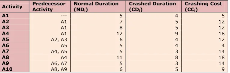
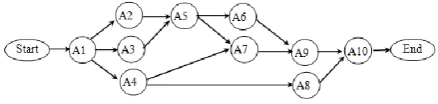
Methodology for crashing of project is illustrated by taking an example of a simple project network. The data pertaining to activities of this project such as requirement of predecessor activities, normal duration, crashed duration (duration in expedited mode), and additional cost needed for executing the activities in expedited mode are given in table 1.

The project has 10 activities and each activity can be done in two ways (modes). The method was applied to select the activity mode of activities to reduce the duration of project network from 35 time units to 30 time units.

Activity Predecessor _Activity Normal Duration _(ND

i)

Crashed Duration (CDi)

Crashing Cost (CCi)

A1 --- 5 4 5

A2 A1 7 5 12

A3 A1 8 5 12

A4 A1 12 9 18

A5 A2, A3 6 4 12

A6 A5 5 4 4

A7 A4, A5 5 3 14

A8 A4 11 8 18

A9 A6, A7 5 3 14

A10 A8, A9 6 5 9

Table 1. Input Data for Activity Crashing of Project Network

Figure 1. Project network diagram showing activities on node

The method was implemented on an electronic spreadsheet by assigning different values to “w” (weight for known parameter). The width of search space is dependent on weight “w”. The activity index for expediting based on assignable parameters and search for a particular weight (w = 0.6) is shown in table 2.

Activity

number Index based on assignable

parameters (Mi)

Search space

Range of Oi for w = 0.6

Random number for particular trial (Ri)

Overall Index for expediting (Oi)

Min Max

1 1.000 0.600 1.000 0.576 0.830

2 0.139 0.083 0.483 0.116 0.130

3 0.417 0.250 0.650 0.967 0.637

4 0.370 0.222 0.622 0.259 0.326

5 0.556 0.333 0.733 0.094 0.371

6 0.417 0.250 0.650 0.003 0.251

7 0.238 0.143 0.543 0.730 0.435

8 0.185 0.111 0.511 0.331 0.244

9 0.238 0.143 0.543 0.451 0.323

10 0.185 0.111 0.511 0.538 0.326

Table 2. Search Space for selection of best solution from trials

The method of generating one solution for w = 0.6 is given in table 3. As shown in table 3, the activity 1, 4, 5, 6, 9 and 10 are to be executed in expedited mode and rest activities to be executed in normal mode. The activity mode of this current solution, EMc may be represented as [1001110011], where 0 represents normal mode and 1 represents expedited mode. The corresponding project duration, PDc is 29 and total cost of crashing TCc is 62.

Iteration

Number Maximum value of Overall Index in each iteration Activity selected for crashing Project duration after crashing Cumulative cost of crashing

Mi Ri Oi

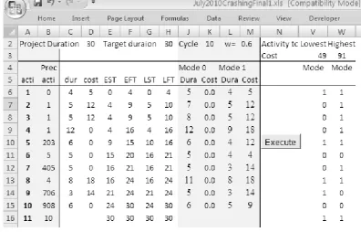
A number of solutions are generated in this manner and the best among them is taken as an efficient solution. The process is easily automated on electronic spreadsheet. The snapshot is shown in figure 2.

Figure 2. Snapshot of implementation on electronic spreadsheet

Activity

Number I Activity Mode of Some Efficient and Inefficient Solutions II III IV V VI VII VIII IX X

1 1 1 0 1 1 1 1 1 0 1

2 0 0 0 0 0 0 1 1 1 1

3 1 0 0 0 0 0 0 0 1 1

4 1 1 1 1 1 0 1 1 1 0

5 1 1 1 1 1 1 1 1 1 1

6 1 0 1 1 0 0 1 1 1 1

7 0 0 0 0 0 0 1 1 1 1

8 0 0 0 0 0 1 1 1 1 1

9 0 1 1 1 1 1 0 1 0 1

10 1 1 1 0 0 0 1 0 1 1

Cost of

crashing 60 58 57 53 49 49 92 97 99 100

Table 4. Some solution generated by simulation in different trials

also obtained in solution-VI by executing activity 1, 5, 8 and 9 in expedited mode and rest activities in normal mode.

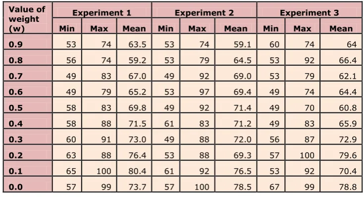
Experiments were done to generate solution for different values of weight of w, by conducting 10 trials in each experiment. The minimum, maximum and mean solutions generated in 10 trials, by taking different values of “w” are given in table 5.

Value of weight (w)

Experiment 1 Experiment 2 Experiment 3

Min Max Mean Min Max Mean Min Max Mean

0.9 53 74 63.5 53 74 59.1 60 74 64

0.8 56 74 59.2 53 79 64.5 53 92 66.4

0.7 49 83 67.0 49 92 69.0 53 79 62.1

0.6 49 79 65.2 53 97 69.4 49 74 64.4

0.5 58 83 69.8 49 92 71.4 49 70 60.8

0.4 58 88 71.5 61 83 71.2 49 83 65.9

0.3 60 91 73.0 49 88 72.0 56 87 72.9

0.2 63 88 76.4 53 88 69.3 57 100 79.6

0.1 65 100 80.4 61 92 76.5 53 92 70.4

0.0 57 99 73.7 57 100 78.5 67 99 78.8

Table 5. Minimum, Maximum and Mean value of cost of crashing generated in experiments consisting of 10 trials

The total cost for crashing the duration of project from 35 to 30 is 49 only. It is seen that the chance of getting efficient solution from limited number of trials is more when weight “w” is in the range 0.4 to 0.7.

8 Validation of Approach

Validation of this approach was done by applying it to number of other sample projects. For illustration purpose, the result of its application on two sample projects is given in table 6.

Project Experiment _Number Lowest cost after 10 trials by using the algorithm Lowest cost after 100 random trials Number trials to get the

minimum cost Number of activities = 19

Normal duration = 169 Target duration = 135 Crashing cost as per solution based on heuristic method = 51

1. (w = 0.5) 2. (w = 0.6) 3. (w = 0.7)

42 49 51

74 Stopped after 1200 trials

Number of activities = 18 Normal duration = 173 Target duration = 155 Crashing cost as per solution based on heuristic method = 38

1. (w = 0.5) 2. (w = 0.6) 3. (w = 0.7)

26 26 30

33 _{Lowest cost} 1092 trials obtained 30

Table 6. Result of Application on two more examples

9 Conclusion

Traditionally, the time-cost problem is addressed by analytical approaches. The analytical method involves lot of computation work. The activity crashing for discrete time-cost function is also known to be NP-hard. So several sophisticated optimization and soft-computing techniques such as Dynamic Programming, Integer Programming, Genetic Algorithm, Ant Colony Optimization etc. that have been used for finding efficient solution to activity modes selection problem. These techniques are quite complex, and are difficult to apply to real life projects that consist of large number of activities.

In this paper, a simple method has been presented for solving discrete time cost trade-off problem by deterministic simulation. The activities are selected for crashing based on some assignable parameters, i.e. criticality of activity and cost effectiveness of crashing. Since selection of activity modes based on assignable parameters does not guarantee optimality, an additional random parameter is introduced and solutions are generated by deterministic simulation. A certain number of solutions (10 to 15) are generated and the best among these is picked up as efficient solution to activity crashing problem.

References

Burns, S.A., Liu, L., & Feng, C.W. (1996). The LP/IP hybrid method for construction time-cost trade-off analysis. Construction Management and Economics, 14(3), 265-276. http://dx.doi.org/10.1080/014461996373511

De, P., Dunne, E.J., Ghosh, J.B., & Wells, C.E. (1997). Complexity of the discrete time/cost trade-off problem for project networks. Operations Research, 45, 302-306. http://dx.doi.org/10.1287/opre.45.2.302

Kelley, J.E. (1961). Critical Path planning and scheduling: Mathematical basis.

Operations Research, 9(3), 296-320.

Moder, J.J., Phillips, C.R., & Davis, E.W. (1983). Project management with CPM, PERT and precedence diagramming (3rd _{Ed). New York: Van Nostrand Reinhold.}

Panagiotakopouols, D. (1977). Cost-time model for large cpm project networks.

Construction Engineering and Management, ASCE, 103(C02), 201-211.

Rahimi, M., & Iranmanesh, H. (2008). Multi objective particle swarm optimization for a discrete time, cost and quality trade -off problem. World Applied Sciences Journal, 4(2), 270-276.

Seal, K.C. (2001). A generalized PERT/CPM implementation in a spreadsheet.

INFORMS Transactions on Education, 2(1), 16-26. http://dx.doi.org/10.1287/ited.2.1.16

Skutella, M. (1998). Approximation Algorithms for the discrete time-cost tradeoff problem. Mathematics of Operations Research, 23(4), 909-929.

http://dx.doi.org/10.1287/moor.23.4.909

Sunde, L. & Lichtenberg, S. (1995). Net-present-value cost/time tradeoff.

International Journal of Project Management, 13(1), 45-49.

http://dx.doi.org/10.1016/0263-7863(95)95703-G

Tareghian, H.R., & Taheri, S.H. (2006). On discrete time, cost and quality trade-off problem. Applied Mathematics and Computation, 181, 1305-1312.

http://dx.doi.org/10.1016/j.amc.2006.02.029

Wiest, J.D., & Levy, F.K. (1977). A Management Guide to PERT/CPM. Prentice-Hall.

Journal of Operational Research, 49(1), 140-152. http://dx.doi.org/10.1016/0377-2217(90)90125-U

Journal of Industrial Engineering and Management, 2011 (www.jiem.org)

Article's contents are provided on a Attribution-Non Commercial 3.0 Creative commons license. Readers are allowed to copy, distribute and communicate article's contents, provided the author's and Journal of Industrial Engineering and

Management's names are included. It must not be used for commercial purposes. To see the complete license