This mine is mine!
How minerals fuel conflicts in Africa
∗Nicolas Berman† MathieuCouttenier‡ Dominic Rohner§ Mathias Thoenig¶
First version: July 2014 This version: June 12, 2015
Abstract. We combine original geo-referenced data on mining extraction of 15 minerals with infor-mation on conflict events at spatial resolution of 0.5◦×0.5◦ for all Africa over 1997-2010. Exploiting exogenous variations in world prices, we find a positive impact of mining on conflict at the local level. Quantitatively, the historical rise in prices (commodity super-cycle) explains 15-25 percent of average country-level violence in Africa. We then document how the appropriation of a mining area by a fighting group contributes to the escalation from local to global violence. Finally, we analyze the impact of corporate practices and transparency initiatives in the mining industry.
JEL classification: C23, D74, Q34
Keywords: Minerals, Mines, Conflict, Fighting, Natural Resources, Rebellion
∗
We thank Gani Aldashev, Chris Blattman, Paola Conconi, Ruben Enikopolov, Nicola Gennaioli, Hannes Mueller, Paolo Pinotti, Uwe Sunde, and Oliver Van den Eynde, and seminar and conference audiences in Montpel-lier, Oxford (OxCarre), Aix-Marseille, ABCA 2015 Berkeley, IEA World Congress Jordan, Universitat Autonoma de Barcelona, Bern, Lyon, Geneva, Uppsala, IPEG Pompeu Fabra, Warwick, Ente Einaudi, Workshop on “The Geography of Civil Conflict” in Munich, the Conference on the “Political Economy of Conflict and Develop-ment‘” in Villars, and the “Workshop on Conflict” at Bocconi University for very useful discussions and comments. Andre Python, Quentin Gallea, Valentin Muller, Jingjing Xia and Nathan Zorzi provided excellent research as-sistance. Mathieu Couttenier and Mathias Thoenig acknowledge financial support from the ERC Starting Grant GRIEVANCES-313327. This paper features an online appendix (available on the authors’ websites) containing additional results and data description.
†
Graduate Institute of International and Development Studies (Geneva) and CEPR. E-mail: [email protected].
‡
Department of Economics, University of Lausanne. E-mail: [email protected]
§
Department of Economics, University of Lausanne and CEPR. E-mail: [email protected].
¶
1
Introduction
Natural riches such as valuable minerals have often been accused of fueling armed fighting. A typical case that recently made the headlines is the heavy fighting that broke out between the Rizeigat and Bani Hussein, two Arab tribes, for the territorial control of the Jebel Amer gold mine in Darfur region, killing more than 800 people and displaced some 150,000 others since January 2013.1 Armed groups extract revenues from mines without necessarily directly managing them, and extorsion or bribing practices have been widely documented in mineral-abundant conflict areas. An example is the financial and logistical support provided by the mining company AngloGold Ashanti in 2003-2004 to the “Nationalist and Integrationist Front” (FNI), a rebel group operating in the gold-rich district of Ituri in Eastern DRC.2
The present paper investigates the impact of mining on conflict by using geolocalized data on conflict events and mining extraction of 15 minerals for all African countries over the 1997-2010 period. Our results show that mining activity increases conflicts at the local level and then spreads violence across territory and time by enhancing the financial capacities of fighting groups. Our empirical analysis is based on the combination of an original dataset,Raw Material Data (RMD), documenting the location and the types of mines and minerals, and Armed Conflict Location
Events Data (ACLED) that provides information on the location and type of conflict events and
the involved actors. The units of analysis are cells of 0.5 × 0.5 degree latitude and longitude (approx. 55km×55km at the equator) covering all Africa. The use of geo-referenced information enables causal identification: Including country×year fixed-effects and cell fixed-effects, we exploit in most of our econometric specifications the within-mining area panel variations in violence due to changes in the world price of the main mineral extracted in the area.
In the first part of our analysis, we estimate the extent of mining-induced violence at the local level. We find a positive effect of mining activity on conflict probability: (i) in the cross-section, this probability is higher in cells with active mines; in the panel (within cells), it increases with mine opening/closing; (ii) a spike of mineral prices increases conflict risk in cells producing these commodities. These results are robust to a variety of consistency checks. We also find that countries with better government effectiveness and with less social cleavages are less affected by mining-induced violence; however, we detect no moderating effect of political institutions (e.g. democracy, rule of law, and voice and accountability). We then perform several quantification exercises to gauge the magnitude of the effect: A one-standard deviation increase in the price of minerals translates into an increase in probability of violencein mining areas from the benchmark 16.7% to a counterfactual 20.1%. When aggregated at the country level, the effect remains
1Fighters from the “Sudan Liberation Army” (SLA) have operated their own illicit gold mine in Hashaba to the
east of Jebel Amer to finance their fighting. Other prominent examples of rebels sustaining their fighting efforts with the cash from running mines include for example rebels groups operating in Sierra Leone and Liberia such as the “Revolutionary United Front” (RUF) that financed weaponry with “blood diamonds” (Campbell, 2002), or the case of Angola’s rebels from “Uni˜ao Nacional para a Independˆencia Total de Angola” (UNITA) that financed their armed struggle with diamond money (Dietrich, 2000). See Reuters, 8 October 2013, “Special Report: The Darfur conflict’s deadly gold rush”. Another typical example is the Marikana Mine Massacre, where in a wildcat strike at a platinum mine owned by Lonmin in the Marikana area, close to Rustenburg, South Africa in 2012 several dozens of people were shot. Cf. BBC, 5 October 2012, “South African mine owner Amplats fires 12,000 workers”.
2Human Right Watch brief, 5 June 2005, “ D.R. Congo: Gold Fuels Massive Human Rights Atrocities”. For
sizeable. We quantify the effect of the historical rise in mineral prices between 1997 and 2010, which according to most scholars was mainly due to the sharp increase in the demand for minerals by emerging market countries such as China and India (Humphreys, 2010; Carter, Rausser and Smith, 2011). Our estimates suggest that the contribution of this so-called commodities super
cycle to the average violence observed across African countries over the period lies between 15
and 25%.
In the second part of the paper we take a more global view and investigate the diffusion over space and time of mining-induced violence, a question of central importance for understanding how local conflicts escalate into regional or national wars. Looking at the nature of violent events, we find that mineral price spikes fuel both low-level violence (riots, protests) and organized violence (battles). The rationales behind each type of violence being different, we focus on battles, that involve 252 rebel groups in Africa over the period, and provide evidence that mines spread conflicts across space and time by making rebellions financially feasible. More precisely, we make use of the information contained in theacleddata on the winners and losers of particular battle
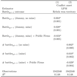
events. We show that the appropriation of a mining area by a rebel group increases the probability that this group perpetrates violence elsewhere in the rest of the country in the following years. Quantitatively, our estimates suggest that every conquest of a mining area more than doubles the subsequent fighting activity of a group. As an alternative empirical strategy, we show that spikes in the price of minerals produced in the ethnic homeland of a rebel group tend to spatially diffuse its fighting operations.
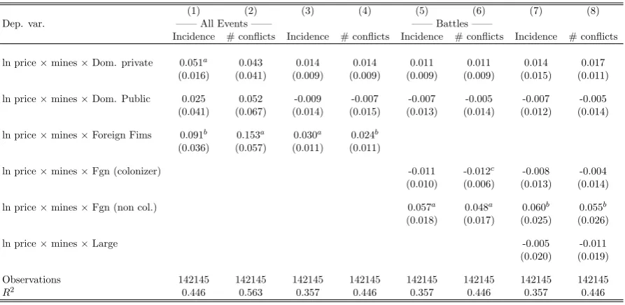
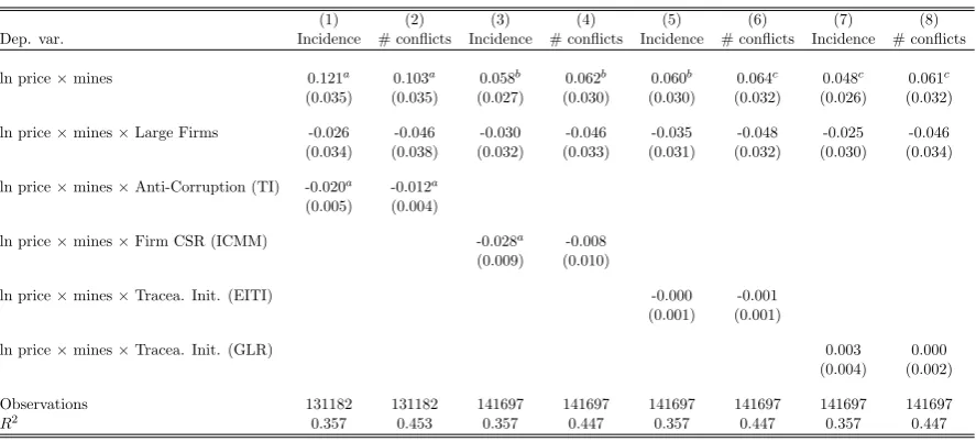
Having documented how mining allows rebel groups to expand their fighting activities, we show in the last part of the paper that the characteristics and behavior of extracting companies is also key. Mining companies have indeed an ambivalent role: On the one hand, they may be willing to secure areas where they plan to operate; on the other hand, they may contribute to the diffusion of violence by financing/bribing rebel groups. We provide suggestive evidence in line with the second channel. Our results show that mining-induced violence is mainly associated with foreign ownership. Nevertheless, among foreign companies, the ones that operate in the least corrupt countries, and the ones that comply to Corporate Socially Responsible practices are asso-ciated with less violence. Finally we evaluate the impact of the recent transparency/traceability initiatives that have been promoted by international agencies, but fail to detect any effect of those top-down policies.
Related literature. In the last ten years there has been an increasing interest of the empirical
literature in linking natural resource abundance to civil conflict and other forms of violence.3 Most existing papers have run pooled cross-country regressions finding that civil war onset and incidence correlate positively with natural resources, generally focusing on oil, diamonds or narcotics.4 The main shortcoming of this “first generation” of papers is that rich and resource-poor countries typically also differ in various geographic, demographic, political and economic
3
Natural resources have also been found to empirically matter for homicides (Couttenier, Grosjean and Sangnier, 2014), for organized crime (Buonannoet al., 2015), for interstate wars (Caselli, Morelli and Rohner, 2015) and for mass killings of civilians (Esteban, Morelli and Rohner, 2015).
4
dimensions, and the risk of omitted variable bias and unobserved heterogeneity makes it hard to give a causal interpretation to such cross-country correlations.
A more recent literature tries to take into account this issue through the use of panel data and the inclusion of country fixed-effects, focusing on variations in prices or resource discoveries as an identification device. This has led to contradictory results: While Lei and Michaels (2014) find a positive effect of oil discoveries on conflict, Cotet and Tsui (2013) find that oil discoveries do not have an effect on conflict anymore when controlling for country fixed-effects. Commodity price shocks also have an unclear effect on conflict, and are found in particular to be unrelated to conflict onsets (Bazzi and Blattman, 2014). One of the reasons for these contradictory results could be that having as unit of observation the country-year level is just too aggregate, as in many countries conflicts are concentrated in particular regions (i.e. think e.g. of the Niger delta in Nigeria or the Kurdish part of Turkey). Given this within-country heterogeneity, aggregating information into a country-year panel may lead to noisy estimates and hence attenuation bias. Recently, some papers have used disaggregated data on natural resources and conflict for one particular country, such as Dube and Vargas (2013) on oil in Colombia; Aragon and Rud (2013) on a gold mine in Peru; and Maystadt et al. (2014) on minerals in the DRC, as well as Sanchez de la Sierra (2015) on coltran and gold in Eastern Congo. However, there does not exist so far a study of the nexus between natural resources and conflict with a panel of disaggregated cells covering all minerals and a whole continent (Africa), as we use in the current paper. This yields a big gain in terms of external validity.
The main drawback of the existing empirical literature is that it has typically been unable to distinguish between different mechanisms or channels of why natural resource abundance mat-ters.5 Theoretically, there are various reasons to expect natural resource abundance to fuel conflict. The first is that resources increase the “prize” that can be seized through the capture of the state – which has been referred to as “greed” or “rent-seeking”. A second possibility is that natural resources make rebellion feasible, i.e. relax financing constraints and make it easier to set up and sustain a rebel movement6. None of these papers, however, presents direct evidence at the disaggregated level. The other mechanisms that have been mentioned by the literature relate to separatism (natural resources provide perspectives of viable independence to resource rich regions with ethnic minorities – Morelli and Rohner, 2013), state capacity (rentier states can rely on resource rents and do not build up enough state capacity, which makes them eventually more instable) and grievances (natural resources can exacerbate grievances, due to frustrations from environmental degradation, or banned access to lucrative mining jobs)7.
In a nutshell, the novelty of our current paper is manifold: First, this is the first paper assessing systematically the impact on conflict of all major minerals. Second, it is the first study of resource abundance and conflict i) using data at a high spatial resolution, ii) covering all Africa and iii) going beyond pooled panel regressions. Third, it is the first study to provide direct, large-scale
5
A notable exception is Humphreys (2005) who uses among others the distinction between production and reserves to distinguish between different channels, running pooled cross-country regressions.
6
See for instance Reuveny and Maxwell (2001), Grossman and Mendoza (2003), Hodler (2006), van der Ploeg and Rohner (2012), Rohner, Thoenig and Zilibotti (2013), and Caselli and Coleman (2013) for the “rent seeking” mechanisms and Fearon (2004), Collier, Hoeffler and Rohner (2009), Nunn and Qian (2014), and Dube and Naidu (2015) for the “feasibility” mechanism.
7See for instance Fearon (2005), Besley and Persson (2011) and Bell and Wolford (2014) on the state capacity
evidence of how capturing a mining area affects the diffusion of conflict over space and time. This yields findings that are in line with the view that resource rents can fuel diffusion of fighting by making it feasible to sustain rebellion. Fourth, we present novel results on how firm characteristics (ownership, Corporate Social Responsibility) can contain or boost mining violence.
The paper is organized as follows: Section 2 presents the data. Section 3 displays the empirical analysis related to the local impact of mining activity on violence. In section 4 we study the diffusion over space and time of mining-induced violence. Section 5 studies the role of mining companies and section 6 concludes.
2
Data
2.1 Data description
The structure of the dataset is a full grid of Africa divided in sub-national units of 0.5×0.5 degrees latitude and longitude (which means around 55×55 kilometers at the equator). We use this level of aggregation rather than administrative boundaries to ensure that our unit of obser-vation is not endogenous to conflict events.8 Our unit of observation is therefore a cell-year in the rest of the paper, i.e. we study how mineral resources affect the probability that a conflict takes place in a given cell, during a given year.
Conflict data. We use the Armed Conflict Location and Event dataset (ACLED, 2013) which
contains information on the geo-location of conflict events in all African countries over the period 1997-2010. We have information about the date (precise day most of the time), longitude and latitude of conflict events within each country. These events are obtained from various sources, including press accounts from regional and local news, humanitarian agencies or research pub-lications. acled records all political violence, including violence against civilians, rioting and
protesting within and outside a civil conflict, without specifying a battle-related deaths thresh-old. A unique feature of theacled dataset is that it contains information on the type of events,
as well as the characteristics of the actors on both sides of the conflicts. We know in particular if the event was a battle, the names of the groups involved, and who won the battle.9 We shall make use of this information when testing for the channels of transmission.
The latitude and longitude associated with each event define a geographical “location”. acled
contains information on the precision of the geo-referencing of the events. The geo-precision is at least the municipality level in more than 95% of the cases, and is even finer (village) for more than 80% of the observations. For each data source, we aggregate the data by year and 0.5×0.5 degree cell. We construct a dummy variable which equals one if at least one conflict happened in the cell during the year, which we interpret as cell-specificconflict incidence, as well as a variable containing the number of events observed in the cell during the year, which we label conflict
8See e.g. La Ferrara and Harari (2014) or Besley and Reynal-Querol (2014) for papers using similar grid-cell
level data combined with the same conflict data.
9Eight different types of events are included in
acled: battle with no changes in territory; battle with territory
intensity. These are our main dependent variables in the rest of the paper. We also show that our results are robust to modeling cell-specific conflict onset and ending separately.
While the geo-coding of the events is cross-checked in theacleddataset, it is not immune to
potential biases and measurement errors. We cannot rule out the possibility that the reporting of conflicts is biased towards certain types of countries, regions or events, as some regions might in particular have better media coverage. An event dataset such asacledcannot, by definition, be
exhaustive. Our empirical methodology makes it however unlikely that this affects our results, as structural differences in media coverage or more generally in the reporting of events will be captured by cell and country-year fixed-effects. We also show that our results are quantitatively stable across events of different severity; this is reassuring as reporting biases are arguably more likely to occur for small-scale events.
Mines data. To each cell-year, we merge information on mines fromRaw Material Data (RMD –
IntierraRMG, 2013). The data contain information on the location of mining companies around the world since 1980.10 We focus on the 1997-2010 period, which overlaps withacled. For each
year, we know whether the mine is active or not, the specific minerals produced and the total production for each of them. We use this data to identify active mining areas, and the type of minerals they produce. For each cell k, we define Mkt, a dummy variable which equals one if a least one active mine is recorded in the cell during year t. As an alternative measure we also compute the number of mines. We also identify the main mineral produced in the cell or by the closest mine, defined as the mineral with the highest production over the entire period. We identify 22 main minerals in our sample of African countries. In the rest of the analysis we focus on the 15 minerals for which we have world price data.11
The RMD dataset collects information mostly for large-scale mines, usually operated by multi-nationals or the country’s government. Hence small-scale mines, and those that are illegally operated, are not included in our sample. While these measurement errors could lead to some attenuation bias in our estimates, we believe that this concern is limited in practice, given our empirical strategy. First, our baseline specification is based on exogenous mineral price variations within cells with a permanently active RMD-registered mine; in other words, the measurement errors are unlikely to attenuate our estimates given the inclusion of cell fixed effects. Second, our unit of analysis being an area (i.e. a 0.5 × 0.5 degree cell) where a mine is active, we interpret our key explanatory variableMktas a proxy for theextraction area of a given mineral rather than as coding for a specific RMD-referenced mine. If minerals are spatially clustered, these mining areas will include all mines, including small ones. Note that we run a number of robustness exercises to ensure that our results are not sensitive to changes in the definition of a mining area. In particular, we include the surrounding cells (first and second degrees) or use 1×1 degree cells instead of 0.5×0.5. As shown later, results are consistent across specifications.
10
More information is available athttp://www.snl.com/Sectors/metalsmining/Def ault.aspx. Other recent research using the RMD data includes Kotsadam and Tolonen (2014) who study gender and local labor market effects of mining, as well as Kotsadam et al. (2015) who assess the impact of mining on local corruption.
11
Other data. Our final dataset contains a number of additional variables. The appendix contains more details on the data construction and sources. In our baseline estimations, we use information on the world price of the minerals from the World Bank Commodities prices dataset. Real prices are measured in constant 2005 USD. We run robustness checks using nominal prices, and alternative commodity prices indices from UNCTAD. We also add diamond prices from Rapaport (2012).12 Finally, we include cell-specific information, including the distance between the cell’s centroid and international borders and to capital city (fromprio-grid - PRIO, 2013),
yearly average level of rainfall and temperature, GDP and population (included inprio-gridbut
originally from G-econ), and satellite nighttime lights from the National Oceanic and Atmospheric Administration (2010) as time-varying proxy for the level of economic activity.
2.2 Descriptive statistics
Figure 1: Conflict events and mining areas
(a)acleddata (b) Mining areas (RMD)
Geo-location of conflict from theArmed Conflict Location and Event dataset (ACLED, 2013) and of active mining areas fromRaw Material Data (RMD). Larger versions of these maps, featuring a distinction between different types of minerals, are provided in the online appendix.
Figure 1 contains a visual representation of both the geo-localization of conflict and mines. The main minerals present in the dataset are gold (30% of mining cells), diamond, copper and coal (around 10% each). As shown in Figure 5 in the appendix, the number of conflict events does not follow a specific trend over time, while the number of active mines is steadily increasing. At the end of the period, our dataset reports around 700 active mines (each possibly producing several minerals).
12
Our final sample contains 52 countries and 15 minerals. Tables 14 and 15 in the appendix contain additional country-level descriptive statistics. On average, around 15 conflict events and 10 active mines are recorded each year in each country. Only four countries display no conflict events over the entire period13, Somalia is the country with the highest number of events (almost 400 events on average by year over the period), while small countries like Burundi, Gambia and Rwanda display the highest share of cells affected by conflict incidence over the period. In 17 countries no active mine is recorded.14 The highest numbers of mines are recorded in South Africa and Zimbabwe, but these are highly concentrated, as in both cases mining areas represent less than 20% of the cells. Note that – except in the case of South Africa – the countries contained in our sample are typically small producers of the minerals from a world perspective: the average market share of a country-mineral is 4.5% (and drops to 1.6% when we exclude South Africa).
Table 1: Descriptive statistics: cell-level
Obs. Mean S.D. Median
Pr(Conflict>0)
all 144690 0.06 0.24 0.00
if mines>0 2771 0.16 0.36 0.00
if mines=0 141919 0.06 0.24 0.00
battles 144690 0.03 0.18 0.00
viol. against. civ. 144690 0.03 0.18 0.00
riots & protests 144690 0.02 0.13 0.00
# conflicts
all cells 144690 0.33 4.238 0.00
if>0 9098 5.23 16.10 2.00
Pr(Mine>0)
only cell 144690 0.02 0.14 0.00
incl. 1stsurrounding cells 140546 0.10 0.31 0.00
incl. 1st&2nd surrounding cells 140546 0.16 0.37 0.00
# mines
all cells 144690 0.05 0.55 0.00
if>0 2771 2.43 3.15 1.00
Pr(# mines>2)
all cells 144690 0.01 0.09 0.00
if mine>0 2771 0.41 0.49 0.00
Source: Authors’ computations from PRIO-GRID, ACLED and RMD dataset.
Table 1 contains descriptive statistics on our final sample, which includes a bit more than 10,000 cells over 14 years. Several elements are worth mentioning. First, the unconditional probability of observing at least one conflict in a given cell and a given year is low at 6%. In the majority of cells no event occurs over the entire period. The probability of observing an active mine in a given cell is also low at 2%, but it increases to 10% (respectively, 16%) when we consider the neighboring cells (respectively, the first and second degree neighboring cells). Second, mines tend to be spatially clustered: conditional on observing at least one mine in a given cell, the average number of mines is 2.43. We can also see this clustering by noting that the probability of observing two mines or more in a given cell, conditional on observing at least on mine is very high
13
Comoros, Cape verde, Mauritius and Sao Tome and Principe.
14
(41%). Finally, the conflict probability is much higher in cells with active mines. Of course, this can be due to many unobserved cell characteristics, an issue we shall deal with in our estimations.
3
Mining-induced Violence: Baseline Results
We turn now to our empirical analysis. We first document correlations between the presence of mining areas and the likelihood of violent events at the cell-level. Then we discuss our strategy for identifying the causal impact of mining on violence and the baseline results are reported. We also provide a series of alternative specifications assessing the robustness of the results. Finally we perform various quantification exercises.
3.1 Correlations
The correlation between mining and cell-level violence is estimated in various ways, all based on specifications of the following form:
conflictkt=α×Mkt+FEk+FEit+Ckt0β+εkt (1)
where (k, t, i) denote respectively cell, time and country. The dependent variable,conflictkt,
corresponds to the observation of violent events at the cell-year level where violence is measured either in term of incidence (i.e. a binary variable coding for non-zero events) or in term of intensity (i.e. number of events). Information on violent events is retrieved from theacleddataset on civil
conflicts. The main explanatory variable,Mkt, measures mining activity at the cell-year level with two possible coding options: a discrete variable equal to the number ofactive mines, or a binary variable coding for the presence of at least one active mine. The vectorFEitcorresponds to a set of country×year fixed-effects that filter out all countrywide time-varying characteristics affecting violence and activity of mines – e.g. a war-induced collapse of central state and property rights.
FEk is a battery of cell fixed-effects and Ckt is a set of potential time-varying co-determinants
of local conflicts and mining activity that includes, in particular, the intensity of violence in the surrounding cells during yeart.
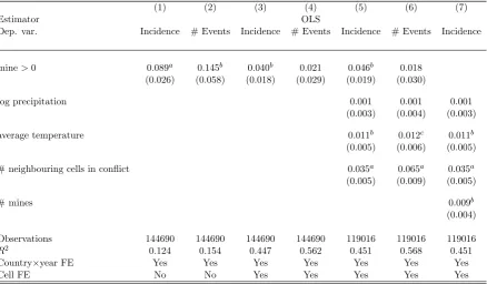
In our baseline specifications, equation (1) is estimated with OLS or LPM in the case of a binary dependent variable. Our results are robust to alternative non-linear estimators such as a conditional logit or a Poisson pseudo-maximum-likelihood estimator (Table A.4 in the online appendix15). In all specifications (here and in other sections of the paper as well), standard errors are clustered at the country-level (note that all our results are robust to less demanding levels of clustering such as country×year or cell). We also check that our main results are robust to a non-parametric estimation of the standard errors allowing for both cross-sectional spatial correlation and location-specific serial correlation (Conley, 1999; Hsiang, Meng and Cane, 2011). Results are displayed in Table 2. In columns (1) and (2) country×year fixed effects are included and the main source of identification corresponds to between-cell variations in mining activity and violence, for a given country in a given year. The presence of one or more mines is associated with a 8.9 percentage points increase in conflict probability. Part of the correlation could be spuriously
15In the online appendix we also consider pure cross-sectional specifications where all variables are averaged in
Table 2: Conflicts and mines: Correlations
(1) (2) (3) (4) (5) (6) (7)
Estimator OLS
Dep. var. Incidence # Events Incidence # Events Incidence # Events Incidence
mine>0 0.089a 0.145b 0.040b 0.021 0.046b 0.018
(0.026) (0.058) (0.018) (0.029) (0.019) (0.030)
log precipitation 0.001 0.001 0.001
(0.003) (0.004) (0.003)
average temperature 0.011b 0.012c 0.011b
(0.005) (0.006) (0.005)
# neighbouring cells in conflict 0.035a 0.065a 0.035a
(0.005) (0.009) (0.005)
# mines 0.009b
(0.004)
Observations 144690 144690 144690 144690 119016 119016 119016
R2 0.124 0.154 0.447 0.562 0.451 0.568 0.451
Country×year FE Yes Yes Yes Yes Yes Yes Yes
Cell FE No No Yes Yes Yes Yes Yes
OLS estimations (LPM for conflict incidence columns). Standard errors, clustered by country in parentheses.csignificant at 10%;bsignificant at 5%;asignificant at 1%.log(x+ 1) used for dependent variables in columns (2), (4), and (6). mine>0 is a dummy taking the value 1 if at least 1 mine is active in the cell in yeart. # mines is the number of active mines in the cell in yeart. # neighbouring cells in conflict is the number of neighbouring cells, among the 8 surrounding cells, in which at least a conflict event occurs in yeart.
driven by omitted time-invariant cell-specific characteristics such as the local determinants of state capacity, property rights enforcement or political instability (e.g. ethnic cleavages). In order to control for this source of unobserved heterogeneity, we include cell fixed-effects in the remaining columns. We obtain a positive and significant (at the 5 percent level) coefficient in column 3, but it loses its significance when violent events at the cell-year level are measured in term of intensity (column 4). In term of magnitude, the within-cell estimates correspond to half of their between-cell counterparts confirming that part of the correlation in column (1) and (2) is driven by time-invariant cell characteristics. Columns (5) and (6) include time-varying cell-specific controls. Despite a substantial reduction in the sample size, our coefficient of interest remains stable and significant in column 5. The opening of a mine in a given cell is associated with a 4.6 percentage points increase in conflict probability in this cell. The coefficient of interest loses significance for explaining the number of conflicts in column 6. Finally column (7) replicates column (5) with the main explanatory variable being the number of active mines in the cell. The coefficient of mining activity is positive and statistically significant at the conventional threshold.
3.2 Exogenous changes in the value of mines – Baseline Results
instance if the state uses part of the mines production to fight insurgency. Guidolin and La Ferrara (2007) actually find evidence that conflicts increase the value of extractive firms.16
In order to address causality, we focus on exogenous variations in the economic value of mines. The idea is that more valuable mines increases local rent-seeking and, consequently, the likelihood of violence.17 To abstract from local determinants of violence and guarantee exogeneity, we exploit the variations in the world prices of minerals. More precisely, we estimate the following specification:
conflictkt=α1Mkt+α2lnpWkt +α3 Mkt×lnpWkt
+FEk+FEit+εkt (2)
The variable pWkt is time-varying and cell-specific and it corresponds to the world price of the main mineral produced by the mines present in cell k, i.e. the one with the highest total production over theentire 1997-2010 period. We codepW
kt as a zero for the cells where no active mine ever produces over the period; by contrast, it is non-zero for cells with a mine that is inactive
only temporary. This coding strategy being non neutral, we check below that our estimates are
robust when restricted to the sub-sample of cells with only permanently active mine.18 Note that we do not include the controls Ckt in our baseline estimations as they reduce significantly the
sample size without affecting the estimates of our coefficient of interest, as shown later in the robustness section.
We are primarily interested in α3, the coefficient of the interaction term between the world price and the dummy for mining activity. This coefficient captures the impact on local violence of an exogenous increase in the world price of a given mineral, in cells where mining extraction of this mineral takes place. Given the fact that we include country×year fixed-effects in all specifications, our identification strategy relies on the exogeneity of the interaction term, Mkt×lnpWkt, with respect to the local determinants of conflict. We discuss hereafter this identification assumption.
a/ Exogeneity of Prices – This seems a reasonable assumption for the world price of minerals,pWkt, as mentioned earlier. Still, one might argue that some mines are large enough to affect world prices, in which case the occurrence of conflict in these cells might also affect these prices. Although our sample contains only few countries with potentially large market power on the mineral market, we nevertheless test whether our results are robust to excluding from the sample all cells located in countries belonging to the top ten world producers of a specific mineral (see subsection 3.3.1).
b/ Exogeneity of mining activity – As discussed above, potential reverse causation from conflicts to mining opening/closing is a severe concern. As a consequence, our coeffi-cient of interest, α3, could be partly identified through conflict-induced shift in the binary variableMkt. To account for this issue, we can restrict the estimate of equation (2) to the sub-sample of cells without opening/closing of mine over the period (i.e. Var(Mkt) = 0 for
16
They mention several reasons that might explain this finding: during conflict, (i) entry barriers might be higher; (ii) the bargaining power of governments might be lower and hence licensing cheaper; (iii) lower transparency leads to more unofficial deals which are profitable to the firms; (iv) the manufacturing sector leaves the country, forcing it to specialize in natural resources.
17See Dube and Vargas (2013) for a similar methodology applied to coffee and oil production in Colombia.
18We also run robustness checks where instead of replacing pW
a given k). Given that Mkt= 0 or Mkt = 1 for all years, this variable is now absorbed by the cell fixed effects and the covariates lnpWkt and (Mk×lnpWkt) become identical; we ac-cordingly include only the interaction term and the specification takes the following simpler expression:
conflictkt=α3 Mk×lnpWkt
+FEk+FEit+εkt (3)
This specification ensures that our coefficient of interest,α3, is identified within cells through the changes in world commodity prices conditional on having apermanent active mine (i.e.
Mkt = 1 for all t), and not through the potentially endogenous opening/closing of mines. Note also that including country×year dummies is crucial, as they absorb common shocks (or trends) on world prices and country-level conflicts. However, from a data perspective, estimating this set of 935 dummies is very demanding. In this respect, keeping in the sample not only cells with a permanent mine opening but also the large amount of cells with no mines (Mkt= 0 for allt) conveys information which is decisive for estimating these dummies. This is why we favor, in our baseline estimations, specifications using the full sample of cells without opening/closing. Alternatively, in the robustness checks, we report the estimates when the sample is restricted to cells with a permanent active mine (see subsection 3.3.4).
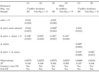
Table 3: Conflicts and mineral prices
(1) (2) (3) (4) (5) (6)
Estimator OLS
Dep. var. Conflict incidence # conflicts Conflict incidence
Sample All Var(Mkt) = 0 All Var(Mkt) = 0 All Var(Mkt) = 0
mine>0 0.042 0.025
(0.028) (0.039)
ln price main mineral -0.042 -0.090b 0.018
(0.027) (0.044) (0.012)
ln price×mines>0 0.109a 0.076a 0.197a 0.101a
(0.037) (0.022) (0.057) (0.032)
# mines 0.009a
(0.003)
ln price×# mines 0.019a 0.026c
(0.006) (0.015)
Observations 143775 142257 143775 142257 144060 142184
R2 0.446 0.446 0.562 0.563 0.447 0.446
Country×year FE Yes Yes Yes Yes Yes Yes
Cell FE Yes Yes Yes Yes Yes Yes
OLS estimations (LPM for conflict incidence columns). Standard errors, clustered by country, in parentheses.csignificant at 10%;bsignificant at 5%;asignificant at 1%. mine>0 is a dummy taking the value 1 if at least 1 mine is active in the cell in yeart. # mines is the number of
active mines in the cell producing the main mineral in yeart. Var(Mkt) = 0 means that we consider only cells in which the mine variable (the
binary version or the number of mines) takes always the same value over the period.log(x+ 1) used for dependent variable in columns (3) and (4). ln price main mineral is the world price of the mineral with the highest average production in the cell over the period. Estimations (1), (3) and (5) include controls for the average level of mineral world price interacted with the mines variables.
consider the number of events. Mines activity is coded as a dummy variable except in columns (5) and (6) where it is measured by the number of active mines in the cell. Columns (1), (3) and (5) are estimated on the full sample (equation 2); while columns (2), (4) and (6) are restricted on the sub-sample of cells without mine opening/closing (equation 3). We see that in all columns but (6), our coefficient of interest is positive and significant at the 1 percent level. Thus, a spike of mineral prices increases the conflict risk in cells producing these commodities. Columns (2) and (4) are our preferred regressions.
3.3 Robustness
In this subsection we show that the baseline estimates of Table 3 are robust to a large battery of sensitivity checks —the main ones relating to exogeneity of world prices, alternative definitions of mining areas and measurement errors in the mining/conflict data. For the sake of exposition most tables are relegated to the online appendix.
3.3.1 Exogeneity of world prices
We start by testing the consistency of our empirical strategy that is based on exogenous variations in world mineral prices. A first threat to our identification strategy could consist in the potential reversed causality from local violence to world prices. In particular, it is conceivable that the occurrence or the anticipation of a conflict in a major producer country leads to an increase in the world prices of the relevant minerals. To address this concern, we drop mining cells belonging to countries that are top-10 world producers of the main mineral produced in the cell. We replicate our baseline Table 3 on this restricted sample with no large producers. Results are statistically robust and quantitatively close to our baseline estimates (Table A.5 in the online appendix).
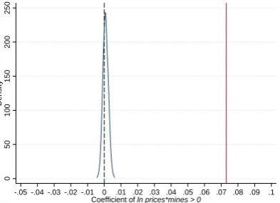
Secondly, we want to rule out the fact that time-varying omitted variables could co-determine world prices and local violence in mining areas. We believe that the inclusion of country×year fixed effects in our baseline specifications alleviates most of this problem. However it could be that the residual unobserved heterogeneity still co-moves with the world prices of minerals. We perform a placebo analysis to exclude this last concern and check the validity of our approach. Our idea is to replace the price of the mineral produced in the cell by the price of a mineral that is
not produced in the cell. More precisely, we randomly assign a mineral to each of the mining cells and run specification (2) of Table 3 with this fake Mkt×lnpWkt variable. We repeat this Monte Carlo procedure in 1,000 draws. Figure 6 displays the sampling distribution of the coefficient of the interaction term. Reassuringly, the Monte Carlo coefficients are distributed far from our baseline estimate (0.076) and are massively insignificant. This confirms that our baseline results are not driven by co-movements in world prices.
3.3.2 Alternative definitions of a mining area
coding for a specific RMD-referenced mine. Imagine now for example that mining areas could on average be larger than our cells of a spatial resolution of 0.5 ×0.5 degree. In this case, focusing on the impact of mines on the conflict likelihood in its surrounding cell of 0.5 ×0.5 degree may underestimate the real impact of being in a mining area. Hence, in what follows we broaden the scope of a mining area.
Table 4: Conflicts and mineral prices, including neighboring cells
(1) (2) (3) (4)
Estimator OLS
Dep. var. Conflict incidence # conflicts
Sample All Var(Mkt) = 0 All Var(Mkt) = 0
mine>0 0.053c 0.037
(0.031) (0.044)
ln price main mineral -0.051c -0.108b
(0.027) (0.045)
ln price×mines>0 0.108a 0.068b 0.197a 0.090b
(0.038) (0.029) (0.057) (0.043)
mine>0 (neighboring cells) -0.028 -0.043
(0.018) (0.031)
ln price×mine>0 (neighbouring cells) 0.020b 0.027b 0.041c 0.047b
(0.010) (0.011) (0.024) (0.021)
Observations 136033 125611 136033 125611
R2 0.442 0.436 0.554 0.551
Country×year dummies Yes Yes Yes Yes
Cell FE Yes Yes Yes Yes
OLS estimations (LPM for conflict incidence columns). Standard errors, clustered by country, in parentheses.csignificant at 10%;bsignificant at 5%;asignificant at 1%. mine>0 is a dummy taking the value 1 if at least 1 mine is active in the cell in yeart. # mines is the number of active mines in the cell producing the main mineral in yeart. Var(Mkt) = 0 means that we consider only cells in which the mine variable
(including the one for surrounding cells) takes always the same value over the period. log(x+ 1) used for dependent variable in columns (3) and (4). ln price main mineral is the world price of the mineral with the highest average production in the cell over the period. All estimations include controls for the average level of mineral world price interacted with the mines variables.
In Table 4 we study the impact on conflict of mineral price shocks in neighboring cells (of degrees 1 and 2) of a cell containing a RMD-referenced mine. As shown by the coefficient of the second interaction term, we detect in all specifications a positive and significant impact, which is consistent with the view that some mining areas are indeed larger than our 0.5 ×0.5 degree cells. Note however that the effect is much lower than for the cell itself (i.e. the first interaction term). Alternatively, in Table A.6 we reproduce our baseline table for a grid of cells at a larger resolution (1 degree ×1 degree).
3.3.3 Measurement Errors
ACLED data. Given that the ACLED data is based on press accounts and news reports, there
may be concerns that media coverage is correlated with mining activity. It could for example be that mining areas have better infrastructure and thus provide easier access to journalists and NGOs. However, as we include cell and country×year fixed-effects, systematic differences in event coverage across mining and non mining areas cannot affect our results. The only reporting bias that would be problematic could arise in case conflict events were more likely to be reported in mining areas during periods of high prices. We cannot rule out this possibility a priori, although we think that it is unlikely that media coverage (typically driven by slow-moving factors such as travel facilities) should be responsive to variations in mining prices (that can be very fast-moving). Still, following Dafoe and Lyall (2015), we run our baseline specifications on different categories of events defined by severity, i.e. by the number of fatalities. The idea is that if there were to be a reporting bias, it should be lower for more severe events: The coefficients for smaller-scale events may be biased downwards but the coefficients for large-scale events should be relatively unbiased (as it is unlikely that any media outlets miss out on big events). We implement this approach in Table A.8 where we estimate the impact of mineral price variations on the probability of conflict for various levels of severity, based on quartiles of number of fatalities. We see that our coefficient of interest is always of the expected sign and statistically significant, even for the highest severity category (which contains events for which the reporting bias should be – if anything – very small). Further, the estimates are quantitatively stable across these different categories of severity, which is at odds with the potential presence of reporting bias. Finally, note that we consider in Section 4 alternative categories of severity, i.e. by types of event, not by fatalities. Here again, the estimates are robust across the different categories. In particular the results hold if we restrict ourselves to battle events, which are very visible and unlikely to be missed out by any news reports.
Mines data. The RMD data only includes big, industrially operated mines, and hence do not
The basic idea consists in gauging the potential impact of non-classical measurement errors by regressing a subsample of our RMD mining data on a quasi-exhaustive list of mines and to see whether the residual variation in RMD coverage can be significantly explained by conflict. The empirical answer is a clear no and we conclude from our exercise that there is no evidence that the RMD data are subject to non-classical measurement errors.
3.3.4 Other robustness checks
Population/economic size and time-varying controls. We want to rule out the fact that our
base-line estimates are driven by an increase in population size resulting from more intense mining activity (induced by raising mineral prices). To this purpose, we control in Table A.10 for eco-nomic size, proxied by night light satellite data, and, more importantly, for the interaction of luminosity and mineral prices. The results are unchanged. Similarly, Table A.11 goes further and includes a number of alternative cell-specific, time-varying controls which might be correlated with commodity price variations (climate variables, such as rainfall and temperature) or mining activity (number of conflicts in the surrounding cells, or number of conflicts observed in the cell since the start of the period). In all cases, our coefficients of interest remain stable and highly significant.
Alternative price data – We also investigate robustness to alternative prices data (Table A.12).
In particular, we use nominal instead of real prices in column (1) and (2), prices from UNCTAD in columns (3) and (4), and replace the price variables by a country-specific index when no mine is ever recorded in the cell in columns (5) and (6).19 In all columns the coefficient of interest is still highly significant and quantitatively close to our baseline estimates.
Subset of metals – Are our results driven by a particular subset of minerals? We respectively
include diamonds in our estimations or exclude gold, silver and diamond mines from our set of minerals (Tables A.13 and A.14).20 Our coefficient of interest keeps its positive sign and is highly significant in all columns, indicating that our results generalize to a broad category of minerals, and that they are not driven by the most precious minerals only.
Sample restrictions –In the baseline specifications cells without mines are included in the sample
with the purpose of estimating the large set of fixed effects (see our discussion in Section 3.2). In Table A.15 we report the estimates when the sample is restricted to cells with a permanent active mine. Column (1) reports our preferred specification on the full sample. Column (2) replicates this specification on the subsample of cells with permanent active mines. The coefficient of interest remains positive but much less accurately estimated, the reason being a massive sample size reduction (1078 observations) with a set of country×year dummies remaining large (280). In column (4), we consequently exclude those dummies and this restores statistical significance. In column (3), for the sake of comparison, we replicate column (4) on the full sample of cells.
19The price series from UNCTAD correspond to weighted indices, calculated from commodity prices tables,
for selected commodities exported by developing economies. The weights used in the construction of the in-dices represent the relative values of exports from developing countries for the period 1999-2001. Data are available at http://knoema.com/UNCTADFMCPI2015Feb/free-market-commodity-price-indices-monthly-january-1960-january-2015.
20
Conflict onset and ending –In all tables we focus on conflict incidence, which reflects our interest in explaining the general presence of conflict. A higher conflict incidence can of course be due to either more conflicts breaking out or due to existing conflicts lasting longer. Hence, in the civil war literature, a number of papers focus on civil war outbreaks (onsets) and endings separately.21 In Table A.16, we study cell-specific conflict onsets and endings of conflict separately. We find that our variable of interest significantly both increases the risk of conflict onset (column (2)), and reduces the likelihood of conflict ending, although the coefficient is less precisely estimated for conflict ending (p-value of 0.117 in column (4)). This suggests that the higher conflict incidence due to mines is both due to more conflicts breaking out and to existing conflicts lasting longer.
Non linear estimators – Table A.17 of the online appendix replicates our baseline specifications
using a class of estimators specifically designed for binary dependent variables and count data, i.e. fixed effects logit (whenever the dependent variable is conflict incidence) or a Poisson pseudo-maximum-likelihood (PPML, whenever the dependent variable is the number of conflict events). Our results are very similar to our baseline estimates. The LPM is however our preferred estimator as it allows for a more straightforward interpretation of the coefficients and does not suffer from certain econometric problems due to the inclusion of both cell and country×year fixed effects.22
Spatial clustering of standard-errors –In all tables standard errors are clustered at the
country-level. Alternatively, we allow for various levels of cross-sectional spatial correlation and cell-specific serial correlation, applying the method developed by Conley (1999) and Hsiang, Meng and Cane (2011). We display the standard errors for our six main specifications when allowing for spatial correlation of 100 or 1000 kilometers, and for a serial correlation over 1 or 5 years (Table A.18). For all combinations of spatial and serial correlation considered, the standard errors are such that our coefficients of interest are still statistically significant at the conventional level.
3.4 Country characteristics and mining induced violence
Is the abundance of valuable mines always a curse for political stability? Countries’ insti-tutions and social characteristics may play a role, as suggested by the rent-seeking models of Mehlum, Moene and Torvik (2006) and Hodler (2006). In particular, minerals could exacerbate instability in countries where the conflict risk is already latently present due to social cleavages or weak institutions. This would be in line with the idea that minerals are not necessarily the deep cause of conflict but make them feasible – a mechanism we shall investigate in detail in the second part of the paper. In this sub-section we consider how country characteristics may modify the average effect of mineral price variations on local conflicts. While asking this question is important, we should be aware that finding strong results would come as a surprise: in most
21A potential issue with using conflict incidence as a dependent variable has recently been raised by the
macro-level literature. Conflict being a persistent variable, one should estimate a dynamic model with the lagged conflict variable included on the right hand side, or equivalently, model onset and ending separately (Bazzi and Blattman, 2014). Note that the problem is less clear in our case as local conflict incidence is much less persistent than country-specific incidence: at the cell-level, the vast majority of events – around 75% – do no last more than 2 years.
22
resource-rich economies in our sample, local heterogeneity in politics and institutions is relatively high and we should not expect strong effects of national characteristics on local violence.
3.4.1 Domestic Institutions: Can Good Governance Stop the Guns?
While natural resources have often been thought of as affecting the nature and quality of institutions (e.g., as generating corruption, autocracies and more generally a weaker accountability of the state), only relatively little attention has been paid to the impact of the interaction between institutional quality and natural resource abundance on political stability and prosperity.23 There are indeed reasons to expect natural resource extraction to have a stronger impact in weak states: it might be easier for local armed groups to extract rents from mining areas in such countries, or the lack of redistribution of mining revenues might create grievances. Starting from our preferred specification (Table 3, column (2)) we now consider the triple interaction between our main explanatory variable (Mk ×lnpWkt) and a country-level index of institutional quality iqi — a binary variable equal to 1 when a country’s institutional score averaged over 1997-2010 is above the sample median.
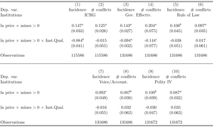
Table 5: Heterogeneous effects: Institutional Quality
(1) (2) (3) (4) (5) (6)
Dep. var. Incidence # conflicts Incidence # conflicts Incidence # conflicts
Institutions ICRG Gov. Effectiv. Rule of Law
ln price×mines>0 0.147a 0.125a 0.143a 0.204a 0.106b 0.097a
(0.033) (0.026) (0.027) (0.075) (0.045) (0.035)
ln price×mines>0×Inst.Qual. -0.084b -0.015 -0.094a -0.144c -0.038 0.017
(0.041) (0.055) (0.032) (0.077) (0.051) (0.061)
Observations 115586 115586 131686 131686 131686 131686
(7) (8) (9) (10)
Dep. var. Incidence # conflicts Incidence # conflicts
Institutions Voice/Account. Polity IV
ln price×mines>0 0.092c 0.087b 0.100b 0.087a
(0.049) (0.038) (0.039) (0.032)
ln price×mines>0×Inst.Qual. -0.016 0.032 -0.030 0.035
(0.055) (0.062) (0.047) (0.063)
Observations 131686 131686 131672 131672
OLS estimations (LPM for conflict incidence columns). Standard errors, clustered by country in parentheses.csignificant at 10%;bsignificant
at 5%;asignificant at 1%. All estimations include country×year dummies and cell fixed effects. log(x+ 1) used for dependent variable in columns (2), (4), (6), (8) and (10). Estimations include cells for which Var(Mkt) = 0, i.e. cells in which the mine variable takes always the
same value. mine>0 is a dummy taking the value 1 if at least 1 mine is active in the cell in yeart. Inst. Qual. is a dummy taking the value 1 if the country is above the sample median of the corresponding variable.
Table 5 displays the results. The dependent variable is the incidence of violence (odd columns) or the number of ACLED events (even columns). In columns (1) and (2), the variable iqi corresponds to theICRG Indicator of Quality of Government(International Country Risk Guide,
23
2013), a standard and synthetic measure of institutional quality at the country-level. In both specifications, the coefficient of the triple interaction is negative, and statistically significant in column (1), while insignificant in column (2). This measure being very coarse, in the following specifications we draw on several more specific indicators of institutional quality, making use of the WGI (“Worldwide Governance Indicators”) dataset from Kaufmann, Kraay, and Mastruzzi (2013).24 We measure iqi with the WGI indicators of Government Effectiveness (columns (3) and (4)),Rule of Law (col. (5) and (6)) andVoice and Accountability (col. (7) and (8)). Finally, in columns (9) and (10) we make use of the standard democracy score of Polity IV (2013). Like the previous indicators, Polity IV scores relate to governance and civil servant behavior; but they also capture the other main dimensions of democracy, i.e. political representation and free elections. In columns (3) and (4), the triple interaction has a negative and statistically significant coefficient suggesting that countries with better government effectiveness are less affected by the political instability induced by mining price shocks. By contrast, we detect no effect for Rule
of Law, Voice and Accountability, and for democracy. These results suggest that institutions
have an ambiguous effect, with government effectiveness reducing the conflict risk, but freedom of assembly and electoral politics having no impact.
3.4.2 Inequality and Diversity: How Does the Social Fabric Matter?
Social cleavages are considered in the literature as important sources of grievances and con-flicts. A natural question consists in assessing whether they also amplify mining-induced vio-lence.25 In the following we consider three alternative variables of social cleavages at the country-level, namely economic inequality, and ethnic and religious fractionalization. As in Table 5, we binarize each of these variables, a one (zero otherwise) coding for a time-average of the variable that is larger than the cross-country sample median.
The results are reported in Table 6. In columns (1) and (2) we focus on the Gini index of gross income distribution of the “Standardized World Income Inequality Database” (Solt, 2014). Higher Gini scores correspond to larger inequality. The positive estimate of the triple interaction term indicates that higher income inequality amplifies the undesirable effect of mining price shocks; the coefficient is significant at the 10% level in column (2) and the p-value is 0.12 in column (1). The next four columns estimate heterogeneous effects with respect to ethnic and religious fractionalization (both variables are from Reynal-Querol, 2014). While the triple interaction with ethnic fractionalization is not statistically significant in columns (3) and (4), we find in columns (5) and (6) that higher religious fractionalization significantly exacerbates the conflict inducing
24The indicators of this dataset are based on a great number of individual variables from 32 data sources. These
individual measures are mapped into clusters of key dimensions of government quality, with higher scores indicating better governance. Government Effectiveness captures “perceptions of the quality of public services, the quality of the civil service and the degree of its independence from political pressures, the quality of policy formulation and implementation, and the credibility of the government’s commitment to such policies”. Rule of Law captures “perceptions of the extent to which agents have confidence in and abide by the rules of society, and in particular the quality of contract enforcement, property rights, the police, and the courts, as well as the likelihood of crime and violence”. Voice and Accountabilitycaptures “perceptions of the extent to which a country’s citizens are able to participate in selecting their government, as well as freedom of expression, freedom of association, and a free media.”
25
Table 6: Heterogeneous effects: Inequality and Diversity
(1) (2) (3) (4) (5) (6)
Dep. var. Incidence # conflicts Incidence # conflicts Incidence # conflicts
Ctry Charac. Gini Ethnic Frac. Religious Frac.
ln price×mines>0 0.025 0.032c 0.069b 0.076a 0.020 0.015
(0.026) (0.019) (0.028) (0.020) (0.033) (0.022)
ln price×mines>0×Charac. 0.074 0.133c 0.018 0.082 0.075c 0.118b
(0.047) (0.078) (0.049) (0.092) (0.043) (0.048)
Observations 108768 108768 127627 127627 127627 127627
OLS estimations (LPM for conflict incidence columns). Standard errors, clustered by country in parentheses.csignificant at 10%;bsignificant at 5%;asignificant at 1%. All estimations include country×year dummies and cell fixed effects. log(x+ 1) used for dependent variable in columns (2), (4) and (6). Estimations include cells for which Var(Mkt) = 0, i.e. cells in which the mine variable takes always the same value.
mine>0 is a dummy taking the value 1 if at least 1 mine is active in the cell in yeart. Charac. is a dummy taking the value 1 if the country is above the sample median of the corresponding variable.
impact of mining price spikes.
3.5 Quantification
How large is the effect of mineral price variations on the conflict probability? In our preferred specification (Table 3, column (2)) a standard-deviation increase in the price of all minerals from their mean translates into an increase in probability of violence from 0.167 to 0.201. This is of non negligible magnitude, but concerns only the cells where active mining takes place. When we also consider the surrounding cells (Table 4, column (2)), conflict probability rises from 0.177 to 0.219.
Over the period of our study mineral prices more than doubled on average.26 For instance, in constant 2005 USD, the ounce of gold was valued at $338 in 1997, and reached $1084 in 2010. This spectacular rise of mineral prices over the 2000-2009 period, known as the2000s commodity boom
or commodities super cycle has attracted quite a lot of attention. There is a consensus among
scholars that no contraction of resource supply is to blame, but rather a rapid and substantial increase in demand, particularly so from the BRICS countries. As pointed out by Carter, Rausser and Smith (2011), “strong global demand, especially in lower-middle-income countries” helped set the stage for this commodity price boom, and “this strong demand was reflected in low real interest rates, a declining U.S. dollar, and strong GDP growth, and it contributed to the reduction in inventory levels that made commodity markets vulnerable to supply and demand shocks” (2011: 107). Similarly, Humphreys (2010) points out that the great metals boom between 2003 and 2008 “can be readily explained by the unusual strength of the demand shock and the lagged response of the supplying industry, with prices receiving an additional boost from the activities of commodity investors” (2010: 1).
What has been the effect of the commodity super cycle on conflicts in Africa? Figure 2 shows, by cell, the predicted decrease in the conflict probability that would be observed in 2010 if the prices were the same as in 1997.27 The regions where conflict probability increases the most
26
More precisely, they have been multiplied by 2.8 in constant USD. Figure A.6 in the online appendix shows the evolution of the price of each of the minerals.
Figure 2: The contribution of rising mineral prices to the probability of conflict in Africa
are Western and Southern Africa. When aggregated at the country level, the magnitude of the effect obviously varies with the number of active mining areas in the country. In Figure 3, we compute, for each country with recorded mines, the contribution to the observed violence of this historical rise in mineral prices (see Figure A.1 in the online appendix for the map equivalent).28 The effect is highly heterogeneous across countries. Averaging across all countries with at least one recorded mine, we find that the historical rise in mineral prices contributed on average to 25% of the observed country-level violence. As is apparent in Figure 3, this number is however inflated by countries, such as Ghana or Mauritania, in which only few conflict events are recorded (see Table 15). When we adopt a more conservative approach and consider only countries with more than 50 events observed over the period, we find that the observed rise in mineral prices
restricted to cells with a permanently active mine over the entire period (Var(Mkt) = 0). Our exercise is based on the in-sample predictions for those cells that we complement with the out-of-sample predictions for cells that have a transiently active mine for which price data is available. Put differently, we apply the estimated coefficients of Table 4, column (2), to all cells contained in Table 4, column (1). Note that a number of cells still do not appear in this map as price data is not available for all minerals.
28This quantification exercise consists in computing the counterfactual share of events that would not have
Figure 3: The contribution of rising mineral prices to violence in Africa
0 .2 .4 .6 .8 1
Share of events explained by increase in mineral prices MRT
GHA BWAMLI ZAF TGOTUN BFATZA BEN NAM SWZ MOZLSO MARCIV GIN ZMB ZWESEN EGY NER RWADZA CODLBR NGA SDNETH SLE KEN AGOGNB BDI
contributed to a 14.5% of the observed violence.29 In the online appendix (Figures A.3.a and A.3.b) we consider a more extreme thought experiment where we quantify the impact on violence of a closing of all mines in Africa. As expected, the effects are even larger: the number of conflicts falls by as much as 60-80% in Zimbabwe or Burkina Faso; and in most countries, the number of conflicts decreases by more than 20%.
We have several reasons to believe that these numbers are conservative estimates. First, our dataset is not exhaustive: only two percent of the cells contain active mines; we consider surrounding cells as well, but many small-scale mines are not included, although they may have a significant impact on violence, adding up to the one we identify here; further, not all minerals are taken into account in these estimations. Therefore, Figure 2 is probably a lower bound of what would be predicted if the same estimations were run on an exhaustive dataset. Second and more importantly, our results only deal so far with the local and contemporaneous impact of mining on violence. In the next section, we emphasize how mining can diffuse violence over space and time, by improving the financial means of armed groups.
4
The diffusion of mining-induced violence over space and time
So far our empirical analysis has focused on local violence, i.e. in the immediate surroundings of mining areas. In this section we take a more global view by investigating the diffusion over space and time of mining-induced violence. The idea is to understand whether mining activity is a factor of escalation from local violence to large-scale conflict. This would be the case if
29Alternatively we can aggregate violenceat the continental level. In that case the contribution of mineral prices
mineral rents finance rebellions, i.e. make rebel movements easier to set up and sustain, or, put differently, make conflictfeasible. The main objective of this section is to test for this mechanism by exploiting the various dimensions of our data – time-series, geo-location, information on the outcome of the violent events, their type, and the identity of the perpetrators.
4.1 The nature of mining-induced violence
From the Wild West to South Africa, there is an abundance of narratives about how dangerous and lawless the mining areas are. They attract a selected subsample of the population, mainly composed of young and uneducated males; labor regulation is often lenient, not to say absent; property rights enforcement is a challenge and this weak institutional environment makes them particularly crime-prone (see Couttenier, Grosjean, and Sangnier (2014) for statistical evidence on homicide rates in US mining areas). By nature, such violence, rooted in riots and protests, is likely to be spatially concentrated around mining areas. By contrast, battles between fighting groups over the control of mines can spread over the space as appropriation relaxes the financing constraints of future fighting capacity. Uncovering the nature of mining-induced violence is thus crucial for understanding whether it can escalate from the local to the global level. Here we provide evidence that different types of events (in terms of scale and objectives) are affected by changes in mineral prices.
Table 7: Minerals price and types of conflict events
(1) (2) (3) (4) (5) (6)
OLS
Sample Var(Mkt) = 0 Var(Mkt) = 0 Var(Mkt) = 0
Dependent conflict var. Battles Violence against civ. Riots / Protests
Incidence # events Incidence # events Incidence # events
ln price×mines>0 0.018a 0.014b 0.046b 0.027 0.041a 0.076b
(0.006) (0.006) (0.023) (0.017) (0.015) (0.030)
Observations 142257 142257 142257 142257 142257 142257
R2 0.357 0.446 0.384 0.499 0.402 0.543
Country×year FE Yes Yes Yes Yes Yes Yes
Cell FE Yes Yes Yes Yes Yes Yes
OLS estimations (LPM for conflict incidence columns). Standard errors, clustered by country in parentheses.csignificant at 10%;bsignificant at 5%;asignificant at 1%. log(x+ 1) used for dependent variable in columns (2), (4) and (6). Var(Mkt) = 0: only cells in which the mine
variable takes always the same value. mine>0 is a dummy taking the value 1 if at least 1 mine is active in the cell in yeart.
In Table 7 we replicate our baseline specifications (columns (2) and (4) of Table 3) for each of the three categories of violent events covered by the acled dataset: battles between fighting
groups, protests/riots, and violence against civilians. As expected, we find that an increase in mineral prices leads to more riots and protests (columns (5) and (6)) and more violence against civilians, though with a less significant coefficient (columns (3) and (4)). More importantly, however, the occurrence of battles is also significantly affected by changes in the value of mines, as shown in columns (1) and (2) confirming that the appropriation of mines is a key driver of violence.30
30