Stratospheric warming influence on the mesosphere/lower thermosphere as seen by the extended CMAM

www.ann-geophys.net/32/589/2014/ doi:10.5194/angeo-32-589-2014

© Author(s) 2014. CC Attribution 3.0 License.

Stratospheric warming influence on the mesosphere/lower

thermosphere as seen by the extended CMAM

M. G. Shepherd, S. R. Beagley, and V. I. Fomichev

Centre for Research in Earth and Space Science, York University, Toronto, Canada

Correspondence to: M. G. Shepherd (mshepher@yorku.ca)

Received: 26 December 2013 – Revised: 16 March 2014 – Accepted: 22 April 2014 – Published: 3 June 2014

Abstract. The response of the upper mesosphere/lower ther-mosphere region to major sudden stratospheric warming (SSW) is examined employing temperature, winds, NOXand CO constituents from the extended Canadian Middle Atmo-sphere Model (CMAM) with continuous incremental nudg-ing below 10 hPa (∼30 km). The model results considered cover high latitudes (60–85◦N) from 10 to 150 km height for the December–March period of 2003/2004, 2005/2006 and 2008/2009, when some of the strongest SSWs in re-cent years were observed. NOX and CO are used as proxies for examining transport. Comparisons with ACE-FTS (At-mospheric Chemistry Experiment–Fourier Transform Spec-trometer) satellite observations show that the model rep-resents well the dynamics of the upper mesosphere/lower thermosphere region, the coupling of the stratosphere– mesosphere, and the NOX and CO transport. New infor-mation is obtained on the upper mesosphere/lower thermo-sphere up to 150 km showing that the NOX volume mixing ratio in the 2003/2004 winter was very perturbed indicating transport from the lower atmosphere and intense mixing with large NOX influx from the thermosphere compared to 2006 and 2009. These results, together with those from other mod-els and observations, clearly show the impact of stratospheric warmings on the thermosphere.

Keywords. Atmospheric composition and structure (middle atmosphere – composition and chemistry)

1 Introduction

The last decade has been marked by a number of very intense major sudden stratospheric warmings (SSW) in the winter Northern Hemisphere, leading to a very per-turbed and dynamically active middle atmosphere. A lot

of attention has been given to the stratospheric warmings which occurred in 2004, 2006 and 2009 (e.g. Manney et al., 2005, 2008a, b, 2009; Funke et al., 2005; Randall et al., 2006, 2009; Hauchecorne et al., 2007; Orsolini et al., 2010; Kvissel et al., 2012) and their effect on the middle atmosphere coupling not only because these SSW events were massive and their effects were felt throughout the middle atmosphere, but also because a number of satellite experiments operating at that time (SABER/TIMED (the Sounding of the Atmosphere using Broadband Emission Radiometry/the Thermosphere Iono-sphere MesoIono-sphere Energetics Dynamics satellite), ACE-FTS (Atmospheric Chemistry Experiment–Fourier Trans-form Spectrometer), Odin/SMR (Sub-Millimeter Radiome-ter), MIPAS (Michelson Interferometer for Passive Atmo-spheric Sounding)/Envisat, GOMOS (Global Ozone Mon-itoring by Occultation of Stars)/Envisat, MLS (Microwave Limb Sounder-Aura)) were able to provide global cover-age of the dynamic response of atmospheric temperature and wind fields as well as various trace gases, to this phe-nomenon.

The SSW is caused by the interaction of planetary waves with the mean flow in the upper stratopause leading to an upward- and poleward-directed heat flux (Matsuno, 1971). According to the World Meteorological Organiza-tion (WMO) definiOrganiza-tion a major stratospheric sudden warm-ing requires that at the 10 hPa pressure level (∼30 km height) or below there are (1) a latitudinal mean temperature in-crease poleward of 60◦_{latitude, and (2) an associated}

590 M. G. Shepherd et al.: Stratospheric warming influence

polar atmosphere from the major SSW is marked by the re-appearance of the warm stratopause layer around its climato-logical position and the slow return of the zonal wind from westward (negative) back to the pre-warming eastward (pos-itive). It takes usually 4–6 weeks for the zonal mean circu-lation to be restored to its pre-warming state. A detailed de-scription of the SSW morphology can be found for example in Schoeberl (1978), Andrews et al. (1987), and Limpasuvan et al. (2004) and the references therein.

Ground-based optical observations of hydroxyl and oxy-gen airglow emission rates and rotational temperatures at high Arctic latitudes (80◦N) in the winter of 2008/2009 al-lowed the examination of the effect of the SSW on these emissions nominally assigned to peak altitudes of∼87 and 94 km, respectively. Shepherd et al. (2010) reported depleted airglow emission rates (by a factor of 7) and a 50–60 K de-crease in the rotational temperatures at the time of the SSW. During the recovery phase the temperatures returned to their pre-event values, while there was an enhancement in the ob-served emission rates. After calibrating the ground-based OH emission rate observations to those observed by SABER it was found that the height of the OH emission rate peak varied from 86 to 91 km at the time of the SSW onset and descended to 78–79 km during the SSW recovery phase.

Modelling of the O volume mixing ratio (VMR), corre-sponding to the observed OH and O2(0, 1) airglow integral emission rates, following the work by Ward (1999) showed atomic oxygen depletion by a factor of∼5 during the SSW that lasted over a number of days. During the SSW recovery phase the O VMR giving rise to the observed O2(0, 1) air-glow emission rates increased by a factor of 3.5 from its pre-SSW level and 17 times from the peak of the pre-SSW, while that of the OH returned to its pre-SSW level. These results sug-gested that at altitudes below∼90 km the effect of the SSW on the mesosphere as seen in the perturbations of the OH peak altitude, airglow emission rates and temperatures was expressed as an upwelling with the airglow layers reaching unusually high altitudes of 91 km for the OH airglow. Pre-ceding the split of the polar vortex, a decrease of the O vol-ume mixing ratio and adiabatic cooling were also observed. A weak downwelling followed, coupled with horizontal mo-tions in the form of 12 and 8 h waves, which restored the O volume mixing ratio to levels comparable to those prior to the SSW event (Shepherd et al., 2010).

The variability seen in the O2atm. emission led Shepherd et al. (2010) to suggest that in the upper mesosphere and lower thermosphere (UMLT) region above 90 km the SSW recovery phase was marked by downwelling and dramatic in-flux of atomic oxygen from the thermospheric reservoir, sig-nificantly increasing the O volume mixing ratio with respect to its pre-SSW state. This infilling overshot the normal levels, increasing the O volume mixing ratio to values∼4 times the normal ones and clearly indicated that the thermosphere was significantly perturbed by the major SSW in January 2009.

The effect of SSW on the upper mesosphere and ther-mosphere was further examined by Shepherd and Shep-herd (2011) employing WINDII (Wind Imaging Interferom-eter) (Shepherd et al., 1993) satellite observations of O(1S) dayglow volume emission rate (VER) in the altitude range from 80 to 300 km and from 50 to 70◦N, observed during the stratospheric warming event in February 1993 (Whiteway and Carswell, 1994; Shepherd et al., 1999; Walterscheid et al., 2000). Of particular interest was the response of thermo-spheric O(1S) dayglow as a proxy for SSW-induced varia-tions in the O volume mixing ratio. The WINDII thermo-spheric O(1S) VER showed a depletion above 140 km in the daytime O(1S) VER, which commenced around the onset of the SSW and lasted over a period of 3–4 days before return-ing to and exceedreturn-ing the pre-SSW values durreturn-ing the SSW recovery phase, an effect similar to that reported by Shep-herd et al. (2010) for the mesosphere and lower thermosphere region at 80◦_{N and consistent with a transport-induced}

de-pletion of O(1S) VER above 140 km, which commenced a little before or around the beginning of the SSW and lasted throughout the SSW event.

Below∼140 km height the fourfold enhancement in the O(1S) VER at ∼100 km was correlated with the temper-ature anomalies of the SSW at the stratopause and in the upper mesosphere as observed by WINDII and reported by Shepherd and Shepherd (2011). Although the SSW in Febru-ary 1993 was far weaker than the recent SSW events from 2004, 2006 and 2009, the direct observations made possible by WINDII for the earlier dates clearly showed the influence of the SSW on the thermosphere, at least up to 200 km. The effect on the thermospheric O VMR for the recent SSW dates would have been much greater as was alluded to by results reported by Shepherd et al. (2010), which is part the motiva-tion behind the current study.

enhanced mesospheric ionization with the enhanced NOX influx from the thermosphere into the mesosphere and up-per stratosphere resulting from energetic particle precipita-tion (EPP) and a strong polar vortex. Energetic (> 10 MeV) solar protons from coronal mass ejections, low-energy elec-trons (1–10 keV) from the magnetosphere during geomagnet-ically disturbed periods, and high-energy electrons (10 keV–a few MeV) from the inner magnetosphere and/or plasma sheet precipitate at polar latitudes and at heights depending on their energy (Turunen et al., 2009). These energetic particles inter-act with the neutral atmospheric gases and change the con-centration of minor tracers like the NOX. During aurora the concentration of NO is directly enhanced by the precipita-tion of low-energy electrons into the lower thermosphere. At high latitudes such enhanced NOX has been observed to descend into the mesosphere and upper stratosphere (e.g. Siskind and Russell III, 1996). Various studies have shown that NOX transport can provide a connection between the ozone observed in the stratosphere and the energetic parti-cle precipitation in the UMLT region (e.g. Solomon et al., 1982; Siskind et al., 1997, 1998). The large NOX in the winter polar region results from the strong downward mo-tion, which advects NOX-rich parcels of air from the winter MLT downward. In the lower thermosphere NOXis produced by photoionization of N2by extreme ultraviolet (EUV) and soft X-rays, while at high latitudes the primary source of NOX is ionizing energetic particle precipitation, from ther-mosphere to stratosphere (Barth, 1992; Barth et al., 1999, 2003; Vitt et al., 2000), while the NOXloss is driven by pho-todissociation. Most of the recent and current satellite ex-periments provide observations below 100 km (MIPAS be-ing an exception with a few selected cases; Funke et al., 2005, 2010), and thus the dynamic response of the thermo-sphere to the recent SSW still remains pretty much unknown. Model simulations of the state of the middle atmosphere dur-ing these SSWs have been predominantly for altitudes be-low 100 km. WINDII still remains the only satellite experi-ment which provided observations of thermospheric oxygen airglow emissions, temperature and winds, but it operated during a period (1991–2003) when no major stratospheric warmings were observed (Manney et al., 2005; Kvissel et al., 2012). The ground-based airglow and temperature obser-vations (Shepherd et al., 2010) showed a SSW effect extend-ing into the UMLT region, but could not provide a compre-hensive picture of the vertical and global extent of the SSW into the thermosphere. To bridge all these observations and examine the stratosphere–thermosphere coupling during the SSWs in 2004, 2006 and 2009 the extended Canadian Mid-dle Atmosphere Model (CMAM) with continuous incremen-tal nudging (CIN) has been employed over the altitude range from 10 to 200 km and the results obtained are presented and discussed in this paper. The paper is organized as fol-lows: Sect. 2 describes the extended CMAM-CIN, Sect. 3 examines the variability of the modelled temperature and wind fields during the three winter seasons of 2003/2004,

2005/2006 and 2008/2009 as well as the CO and NOX as proxies for transport. The results obtained are discussed in Sect. 4 in the context of available experimental data, and the conclusions are summarized in Sect. 5.

2 The extended CMAM-CIN

The extended CMAM (Beagley et al., 2000; Fomichev et al., 2002; McLandress et al., 2006; Beagley et al., 2010) is one of the first ground-to-thermosphere general circulation models in the world and is based on the regular version of the CMAM described by Beagley et al. (1997). The primary rationale for the extended CMAM is to examine the nature of the phys-ical and dynamphys-ical processes in the mesosphere/lower ther-mosphere region without the artificial effects of an imposed sponge layer which can modify the circulation in an unreal-istic manner. It gave the capability of modelling the physics and dynamics of the atmosphere from the ground to approxi-mately 250 km, thus providing a powerful tool for compar-isons with satellite observational data like those from the Upper Atmosphere Research Satellite (UARS) and the Ther-mosphere Ionosphere Mesosphere Energetics and Dynamics (TIMED). The most recent version of the extended CMAM (Beagley et al., 2010) has incorporated neutral and simplified ion chemistry, actively simulating 99 % of the atmosphere’s constituents except for noble gases which are specified.

The model version used in the current study employs a T47 spectral truncation, with a Gaussian collocation grid of 96×48 points and with 95 levels in the vertical that extend from the ground to 2×10−7_{hPa (200–300 km depending on} the phase of the solar cycle). This corresponds to a horizon-tal resolution of about 4◦ _(3.75◦_{) and a vertical resolution}

592 M. G. Shepherd et al.: Stratospheric warming influence

Table 1a. Photoionozation processes in the extended CMAM.

Reaction J∞ References

O2+hν →O +

2+e 4.94×10

−7 _{Solomon and Qian (2005)}

O2+hν →O++ O +e 1.21×10−7 Solomon and Qian (2005) N2+hν →N+2+e 3.62×10

−7 _{Solomon and Qian (2005)}

N2+hν →N++ N +e 2.78×10−8 Solomon and Qian (2005) O +hν →O++e 2.51×10−7 Solomon and Qian (2005) N +hν →N++e 2.08×10−7 Samson and Angel (1990)

representing N+, NO+and O+and their interaction with the neutral atmosphere over a vertically limited domain. Totally, the model chemistry scheme includes 49 neutral species, 5 ions (NO+, O+, N+, N+₂, O+₂)and electrons, and it employs 102 neutral, 27 ion and 49 photolysis reactions. The nitro-gen chemistry in the extended CMAM is based on the strato-spheric CMAM nitrogen chemistry and expanded. The ex-tended CMAM chemistry no longer treats molecular oxygen and nitrogen as inert fixed fields but advects and introduces chemistry and physics, thus allowing the breakdown of O2 and N2 into O, NO, NO2 and N in the upper atmosphere. The chemistry for molecular oxygen is solved explicitly and combined with the other chemical equations. The atomic ni-trogen is no longer solved using photochemical equilibrium but solved as part of the Newton solver with a large number of new N production and sink terms added, principally re-sulting from the addition of basic ion chemistry (Tables 1a, b). The ion chemistry is a simple subset without electroni-cally excited states considered that provides a good represen-tation of the MLT region but does not represent the chemistry above the lower thermosphere. One recent change in the ex-tended CMAM is the use of the model in a “nudged” mode, which allows the model to be forced towards re-analysis data (ERA-Interim, ERAI; Dee et al., 2011) to study scific events, such as SSW during particular observation pe-riods. The simplified assimilation system of ERAI data em-ploys a CIN scheme, which is based on the incremental anal-ysis updating methodology (Bloom et al., 1996; Polavarapu et al., 2004) to force the lower atmosphere (ground to 10 hPa,

∼30 km) to the observed state. This allows the upper atmo-sphere to be driven by a realistic lower atmospheric state in the form of “forecast” mode with an update frequency of 6 h. The CIN scheme is currently used for atmospheric initializa-tion of the coupled forecast models in the Canadian Seasonal to Inter-annual Prediction Scheme (CanSIPS) (Merryfield et al., 2013). With the CMAM-CIN modelling system the spe-cific dates covering the SSW of 2004, 2006 and 2009 can be modelled and compared to daily observations without the need to resort to climatological comparisons.

The mesospheric response to the three recent major SSWs in the winters of 2003/2004, 2005/2006 and 2008/2009 has been the focus of many observational studies. As it will be shown hereafter, although the model was nudged only up to 10 hPa (∼30 km), the extended CMAM-CIN captures

Table 1b. Ion chemistry reactions used in the extended CMAM

Reaction Reaction coefficient Reference

O+₂+ NO→NO++ O2 4.6×10−10 Woodall et al. (2007) O+₂+ N2→NO++ NO 5.0×10−16 Rees (1989) O+₂+ N→NO++ O 1.8×10−10 Woodall et al. (2007) N+₂+ O₂→O+₂+ N₂ 5.0×10−11 Woodall et al. (2007) N+₂+ NO→NO++ N₂ 4.4×10−10 Woodall et al. (2007) N+₂+ O→NO++ N 1.3×10−10 Woodall et al. (2007) N+₂+ O→O+_{+ N}

2 1.0×10−11 Woodall et al. (2007) N+₂+ N→N++ N2 1.0×10−11 Woodall et al. (2007) O++ O2→O+2+O 1.9×10

−11 _{Woodall et al. (2007)}

O++ N2→NO++ N 1.2×10−12,∗ Woodall et al. (2007) N++ O2→NO++ O 2.63×10−10 Woodall et al. (2007) N++ O2→O++ NO 3.66×10−11 Woodall et al. (2007) N+_{+ O}

2→O+2+ N 3.11×10

−10 _{Woodall et al. (2007)}

N++ NO→NO++ N 4.51×10−10 Woodall et al. (2007) N++ NO→N+₂+ O 7.90×10−11 Woodall et al. (2007) N++ O→O++ N 5.0×10−13 Woodall et al. (2007) e+ O+₂→2 O 1.06×10−5T−0.7 Woodall et al. (2007) e+ NO+→N + O 3.55×10−6T−0.37 Woodall et al. (2007) e+ N+₂→2 N 9.41×10−7T−0.30 Woodall et al. (2007) e+ O+→O 1.40×10−10T−0.66 Woodall et al. (2007) e+ N+→N 1.09×10−10T−0.58 Woodall et al. (2007)

∗_{T> 223 K}

realistically the mesospheric response to these events through the model dynamics and this agreement serves to validate the consistency in the thermospheric dynamical response to SSWs while examining the coupling of the thermosphere with the middle atmosphere.

3 Results

3.1 The winter Arctic middle atmosphere

Model simulations of temperature, zonal and meridional winds, NOX and CO have been examined for the period from December to March of 2003/2004, 2005/2006 and 2008/2009, over the altitude range from 10 to 200 km and latitudes from 50 to 85◦N. The evolution of the zonally av-eraged temperature and the mean zonal wind from 10 to 150 km height at the time of the major SSW events (observed on 23 December 2003, 21 January 2006 and 23 January 2009, or day of year 360, 385 and 387 starting from January 1 of 2003, 2005 and 2008, respectively) is shown in Figs. 1– 3. Figures 1 and 2 present the temperature evolution at 80 and 65◦_{N, respectively, while Fig. 3 shows the zonal winds}

at both 80 and 65◦_{N latitude. For each of the three winter}

effect of the large vertical temperature gradients throughout the altitude range of the UMLT region. The upper and bot-tom panels overlap in height at 100–110 km in order to map corresponding signatures between the two regions, the strato-sphere/mesosphere and the lower thermosphere. According to the model results, most pronounced at 80◦N, there was a stratospheric warming event around 23 December 2003 (day of year 355–358, beginning 1 January, Fig. 1b) with zonal mean temperature of ∼275 K at 45 km height (the stratopause), which was accompanied by cooling of the up-per mesosphere from∼75 to∼100 km due to adiabatic ex-pansion and vertical advection at the time of the SSW as was first noted by Labitzke (1972), and further discussed by Siskind et al. (2005) and Cho and Shepherd (2006). This mesospheric cold temperature anomaly has a down-ward phase progression suggesting upwelling at the time of the SSW. An anomalous descent can be seen below 100 km down to 30 km around day 360, with a mesospheric cold tem-perature anomaly appearing almost simultaneously above the stratospheric warm temperature anomaly associated with the SSW. During the recovery phase, day 365–385 (1–20 Jan-uary 2004), there was an increase of temperature in the meso-sphere around days 375 and 380 (10 and 15 January 2004) associated with the reformation of the stratopause. The stratopause reformed around day 380 at ∼70 km, but was colder than prior to the SSW event and remained cold un-til day 410 (14 February 2004) before descending to about 60 km for the rest of February 2004. It further warmed up and slowly descended with a rate of∼200 m day−1, which is considered a normal vortex descent rate. The UMLT region above 90–100 km height remained undisturbed after day 390 (25 January 2004). This was consistent with experimental re-sults discussed by Manney et al. (2005) and is not observed in the model results for the other two winter seasons con-sidered (Fig. 1c, d, e and f). At the time of the SSW and the mesospheric cold anomaly in late December 2003 and early January 2004 an enhancement in the residual tempera-ture in the lower thermosphere around day 360 (25 Decem-ber 2003) was observed right above the mesospheric cold anomaly at the beginning of the recovery phase following the stratospheric warming (Fig. 1a). It peaked at 110 km with 25 K and extended up to at least 150 km with residual val-ues of 10 K throughout the altitude range. A weaker tem-perature anomaly with a peak of 10 K at 110 km was also extended into the lower thermosphere around days 375–380 (10–15 January 2004). At the time of the cool stratopause from days 380 to 410 (15 January to 14 February 2004) a cold thermospheric anomaly settled above 105–110 km and lasted till the end of February (∼day 425).

In 2006 (Fig. 1c, d) a SSW onset occurred around day 375 (10 January 2006). The stratopause broke up, setting off a recovery phase, which continued until day 400–405 (4– 9 February 2006), when the restored stratopause was well into the climatological mesosphere, reaching as high as 75–80 km. Temperatures of 200 K reached what would be the

climatological upper mesosphere and the mesopause region, at∼95 km. The warming of the mesosphere was observed for about 5 days as high as 100 km, destroying the mesopause before the mesosphere and the mesopause gradually returned to their seasonal temperatures by the end of March 2006. The stratopause descended with a rate of∼600 m day−1between days 400 and 430 (4 February and 5 March 2004).

The stratospheric warming and the cold mesospheric anomaly in January 2006 (around day 380, 15 January) were accompanied by a thermospheric warming with a peak of 20 K at ∼110 km (Fig. 1c,d), while the effect of the stratopause recovery phase and the elevated stratopause were accompanied by a cold thermospheric anomaly, which ex-tended up to 150 km height and lasted till the end of Febru-ary (about day 420). In 2008/2009 (Fig. 1e, f) an early stratospheric warming was observed around day 340 (the beginning of December 2008), with a brief recovery phase around day 350 before strengthening again with a second major SSW triggered around day 380 (15 January 2009). The stratopause descended to as low as 30 km (240 K con-tour) on day 385 (20 January 2004), with a warm temper-ature of 230 K extending even further down to the lower stratosphere. The recovery phase lasted for about a week, and by day 400 (4 February 2009) the stratopause was re-formed at what would normally be considered climatologi-cal upper mesosphere at∼90 km, practically destroying the mesosphere, as it was during the SSW 2006. Over the next two months the stratopause gradually returned to its climato-logical altitude at 50 km.

As in the previous cases, the cold mesospheric anomaly at the time of the January 2009 (around day 390, 25 January) SSW was accompanied by a thermospheric warm anomaly (Fig. 1e) with a peak of 20 K at 110 km and extending up to 140 km height with a value of 10 K. The effect of the elevated and reformed stratopause extended up to 110 km (Fig. 1f). The cold thermospheric anomaly closely mapped the refor-mation and the strengthening of the stratopause, with down-ward descent indicating upwelling with adiabatic cooling at the time of the stratopause descent toward the last strato-spheric warming at the end of March. From the three win-ters the thermosphere in 2006 appeared quieter over the pe-riod considered with smaller variations around the average, while 2004 was the most disturbed, with variations of at least

±25 K from the average from December to March. The ther-mospheric response to the onset of the SSW and the follow-ing recovery phase appeared as cold temperature anomalies, extending in altitude to at least 150 km into the thermosphere, although the restored stratopause in 2004 was much cooler and lower in peak height than those for either 2006 or 2009.

594 M. G. Shepherd et al.: Stratospheric warming influence

Figure 1. Evolution of the zonal mean temperature at 80◦N for the period 1 December–31 March (day of year 335–455, starting 1 Jan-uary 2003 (2005 and 2008, respectively)) for the three SSW events considered. (a, c, e) Temperature residuals (values averaged over 1 December–31 March are subtracted) from 100 to 150 km; (b, d, f) zonal mean temperatures from 10 to 110 km (5 K contours).

reformation to the climatological height in 2009 was esti-mated to be∼800 m day−1.

At 65◦N, the latitude considered by Shepherd and Shep-herd (2011) (Fig. 2), the three SSWs could be seen in the stratosphere/mesosphere (Fig. 2b, d, f), but similar to the re-sults at 80◦N the thermospheric response was strongest in 2003/2004, spanning a range of 50 K, while in 2006 and 2009 it was less perturbed and about a factor of 2 weaker (Fig. 2a, c, e). The recovery phase of the SSW 2004 was short with no elevation of the stratopause during its reformation (Fig. 2b). From the three seasons considered the SSW 2009 recovery phase was the most prolonged with about 20 days of almost isothermal stratosphere/mesosphere temperature variation of

∼5–10 K from 20 to 80 km (Fig. 2f).

While the altitude of the stratopause prior to the SSW in all three cases was at∼50 km, following the recovery phase it was reformed at an increasing altitude from year to year. For example the 230 K contour can be seen at 70, 80 and 90 km

on day 380 (15 January) in 2004, day 402 (6 February) in 2006 and day 405 (9 February) in 2009, respectively.

The warming seen in the mesosphere/lower thermosphere around 100–120 km height at the time of the SSW on-set is consistent in magnitude with the TIME-GCM/CCM1, GAIA2 and HAMMONIA3 model simulations by Liu and Roble (2002), Liu et al. (2013) and Miller et al. (2013), respectively, and ground-based radar (e.g. Hoffmann et al., 2007; Kurihara et al., 2010) and the MIPAS satellite obser-vations (Funke et al., 2010).

The model zonal mean winds for the three periods of in-terest at 65 and 80◦N are shown in Fig. 3. It can be seen that during the three winter seasons of interest the polar vortex

1_{Thermosphere, Ionosphere, Mesosphere and Electrodynamics}

General Circulation Model/Climate Community Model version 3.

2_{Ground-to-topside model of Atmosphere and Ionosphere for}

Aeronomy.

Figure 2. The same as in Fig. 1, but at 65◦N.

winds were by a factor of almost 2 stronger over 65◦N than at 80◦N. The reversal of the zonal mean wind from eastward direction (positive) to westward direction (negative) in the stratosphere at 65◦N (Fig. 3a, c, e) marked the beginning of the SSW and was also observed at 80◦N (Fig. 3b, d, f) albeit with reduced strength.

In December 2003 at 65◦N and about day 355 (20 Decem-ber 2003, Fig. 3a) the direction of the zonal wind reversed from eastward to westward in the stratosphere as the vor-tex broke down, while the mesospheric winds were all west-ward except for a weak reversal to eastwest-ward (∼10 m s−1)at

∼80–100 km during the SSW recovery phase. The vortex re-formed by day 380 (15 January 2004) with a peak at 60 km at 65◦N (where the restored stratopause was also observed) and at around 65–70 km at 80◦N (Fig. 3b), well into the cli-matological mesosphere. Except for a brief weakening of the eastward winds around day 390 (25 January 2004) it con-tinued building up with a series of warming pulses through-out February and March 2004 (days 400–440, 5 February– 15 March 2004) (Fig. 3a), when the wind speed at 65◦N reached 70–90 m s−1. In the UMLT the prevailing wind was

westward with a peak at 100 km. The warming pulses of increased eastward flow in the stratosphere were accompa-nied by an increase in the westward winds in the UMLT re-gion. The westward winds dominated the recovery phase of the stratopause and extended up to 80 km. They also domi-nated the 80–120 km altitude range (the MLT region) both at 65 and 80◦N except for a brief reversal to eastward winds around days 360–380 (25 December 2003–15 January 2004) during the vortex recovery phase.

In 2006 at 65◦_{N (Fig. 3c) the reversal of the zonal mean}

596 M. G. Shepherd et al.: Stratospheric warming influence

Figure 3. Evolution of the zonal mean wind at 65◦N (left column) and 80◦N (right column) for the period 1 December–31 March (day 335 to day 455), for 2003/2004, 2005/2006 and 2008/2009 (10 m s−1contours).

reforming and descending. The zonal mean wind field at 80◦_{N (Fig. 3d) shows the same pattern, although it is}

gener-ally weaker in strength. The magnitude of the eastward zonal winds at 80–120 km height was comparable to that of the vor-tex at 50 km, prior to the vorvor-tex breakdown. The zonal mean flow reversed back to westward in the UMLT after day 395– 396 (1 February 2006) and remained so until the end of the period considered. The vortex recovery phase at 55 km lasted from day 370 to day 395 (Fig. 3d). The 2006 vortex contin-ued descending and strengthening as it was reforming, with its upper boundary well into the upper mesosphere,∼80 km, and by the first half of March (day 435, 10 March 2006) its lower edge reached 15 km height. The vortex was stronger than the one in 2004 with a peak wind velocity of 90 m s−1 at 65◦N and 55 m s−1at 80◦N.

The modelled zonal wind field during the 2005/2006 SSW shown in Fig. 3c and d is consistent with the MLS and SABER observations at 70◦_{N discussed by Manney et}

al. (2008b) (their Fig. 3) and the MF and meteor radar obser-vations reported by Hoffmann et al. (2007). Both Manney et

al. (2008b) and Hoffmann et al. (2007) reported the onset of the SSW 2006 was preceded by planetary wave 1 amplifica-tion, which coincided with the first wind reversal, and larger amplitude of planetary wave 2 at the onset of the SSW, start-ing the prolonged wind reversal. The short-term reversals of the mesospheric winds were followed by a period of strong eastward winds correlated with enhanced turbulent rates and an increase in the gravity wave activity at 70–85 km height.

beginning to descend over the next two months to∼60 km with a peak wind velocity of 100 and 85 m s−1 _{at 65 and} 80◦_{N, respectively, in early March in the MLT region. The}

prevailing westward winds peaked at∼100 km, and their ef-fect seems to extend well into the lower thermosphere. Above

∼80 km to 100–110 km, the prevailing winds were westward for more than a month, leading to low wave activity and en-abling the formation of a strong polar vortex which did not break until the end of March. Above 120–130 km the zonal mean winds were all eastward.

With the basic fields of temperature and zonal wind de-scribing the dynamical state of the atmosphere during the three SSW seasons, the SSW effects on the trace gases CO and NOXare considered next. Both the temperature and the zonal mean winds predicted by the CMAM-CIN are consis-tent with the SSW climatology of Liu and Roble (2002).

3.2 CO

Measurements of carbon monoxide (CO) have become an important tool for examining large-scale mesospheric circu-lations (Clancy et al., 1984; de Zafra and Muscari, 2004; Grossman et al., 2006) and the vertical motions in the strato-sphere and mesostrato-sphere (Allen et al., 1999, 2000; Forkman et al., 2005; Clerbaux et al., 2005). In the stratosphere and mesosphere CO has long been used to infer dynamical pro-cesses and diagnose trace gas transport (e.g. Hays and Oliv-ero, 1970; Allen et al., 1981). CO is also used to evaluate the dynamics in three-dimensional models (e.g. Jin et al., 2005, 2009; Minschwaner et al., 2010; Kvissel et al., 2012). Dur-ing polar night CO losses are reduced due to the decrease in OH (from reduced photolysis of H2O), which makes its chemical lifetime much longer. In this case CO follows the meridional circulation toward the winter hemisphere polar night pole with strong descent at high latitudes through the mesosphere and stratosphere. As a result, the meridional cir-culation transports high amounts of CO into these regions, which in turn leads to a sharp CO gradient down to the strato-sphere (Solomon et al., 1985), and the downward tilt of the CO isopleths toward spring time. Due to the photodissocia-tion of CO2in the UMLT region there is a large reservoir of CO there with a peak at∼110 km, which can be transported down into the mesosphere and stratosphere during periods of strong descent like the one which occurs during stratospheric warming events (Solomon et al., 1985; Allen et al., 2000).

Figure 4 shows the daily zonal mean CO VMR at 65 and 80◦_{N for the period of day 335 to day 455 (1}

Decem-ber to 31 March) for the three winter seasons considered, 2003/2004, 2005/2006 and 2008/2009 at altitudes from 30 to 90 km. The VMR in ppbv are expressed in terms of log10due to the large VMR vertical gradient observed from the strato-sphere to the thermostrato-sphere. It can be seen that on the dates of the onset of the SSW (day 355 (21 December) in 2003/2004, day 378 (13 January) in 2005/2006 and day 385 (20 January) in 2008/2009) the descent of CO into the winter stratosphere

due to the meridional circulation is interrupted by uplifting of the CO layer, with CO-poor air entering the lower clima-tological mesosphere at and above 60 km, followed by de-scent into the stratosphere, reaching its lowest altitude about 40 days after the SSW event. At 65◦N (Fig. 4a, c, e) the de-scent was stronger in 2004 and 2006, reaching down to 50 km height (e.g.−0.2 contour), while in 2009 it was quite shal-low and comparable to the level prior to the SSW event. At 65◦N the response of the mesosphere to the SSW was more comparable in 2004 and 2006 than in 2009.

At 80◦N (Fig. 4b, d, f) the uplifting at the time of the SSW was more pronounced up to∼70 km in 2004 than in 2006 and 2009. It began at the onset of the SSW and lasted through the recovery phase before the downward funnelling began with the reformation of the elevated stratopause and the reversal of the stratospheric jet back to eastward. A de-scent of CO followed all three SSW events, reaching the stratosphere within about 40 days after the SSW, with fun-nelling of the CO down to about 45–50 km into the strato-sphere (e.g. −0.2 contour). Although this funnelling was massive, its lower border exhibited larger variation in its de-scent, while its temporal extent indicated a connection to the reformation of the polar vortex following the SSW event and the unusually cold stratopause in late January/mid-February 2004, seen in Fig. 1b. In 2004 the recovery phase of the polar vortex at 80◦N was accompanied by a strong down-ward flux (to∼55 km) around days 375–380 (10–15 Jan-uary 2004). After the initial descent immediately following the stratopause recovery phase, around days 380–390 (15– 25 January 2004), no more downward transport appears to take place, but rather the CO funnel is eroded over time, be-ing subjected to horizontal mixbe-ing and loss as the vortex is weak (Fig. 3b) and the advection is decreased (Fig. 4b). The CO flux further descended down to∼45 km over a period of about a month, while gradually being dissolved by more intense vertical mixing during February (days 396–425) and eventually destroyed in early March due to CO losses in reac-tion with OH, formed through H2O photodissociation during the polar sunrise. The relatively flat isopleths above 80 km in the winter mesosphere after day 395 (days 396–455, Febru-ary/March 2004) indicate that equilibrium between vertical transport and horizontal mixing was established quickly and was maintained.

The period between day 380 and 420 (15 January– 24 February 2004), when a weak CO downwelling was ob-served (Fig. 4a, b), coincided with the reforming of the unusually cold stratopause following the SSW recovery phase. Although the stratopause was elevated, it reached only

598 M. G. Shepherd et al.: Stratospheric warming influence

Figure 4. Evolution of the zonal mean CO (log10of VMR in ppmv) at 65◦N (left column) and 80◦N (right column) from 1 December to

31 March (day 335–455) of 2003/2004, 2005/2006 and 2008/2009, for the altitude range 30–90 km.

CO descent appeared massive and very constrained down to

∼45 km, with a strong and long-lasting influx coming from well above 90 km (Fig. 4c, d); it results from the pull of the strong vortex which brings CO air down to the reformed stratopause, where it is mixed with stratospheric air. In the mesosphere CO decreased and eventually was destroyed by the polar sunrise, mixing with meridionally transported mid-latitude low-CO air, and the last stratospheric warming in late March (Fig. 4d). The pattern is similar for the CO down-welling in the winter of 2009 (Fig. 4e, f) which started around day 400 (5 February 2009) – it was broad and long-lasting, with a large gradient at ∼50 km. It dominated the entire range from 50 to 90 km (and above), with a significant reduc-tion in the middle and upper stratosphere after mid-January due to the SSW; it was slowly destroyed through mixing and H2O photodissociation by the end of March. As the recovery phase was short, about a week compared to the 20–25 days in 2004 and 2006, large CO VMRs were still observed in the stratosphere until the end of March 2009.

3.3 NOX

Figure 5. The same as in Fig. 4, but for NOX(NO + NO2)(log10of VMR in ppbv).

months before being destroyed in the upper stratosphere and lower mesosphere through horizontal and vertical mixing and photolysis by sunlight resulting from the polar sunrise.

An increased vertical and horizontal mixing is most ap-parent at 80◦_{N in 2004 (Fig. 5b), with an influx around}

day 380, after which the NOX VMR was rapidly mixed and remained at about the same level over the next 40 days, be-fore being destroyed by mid-March. There is a prolonged descent of NOXfrom the UMLT region down to about 75– 80 km following the influx on day 380 (15 January 2004), but it did not penetrate further down into the lower meso-sphere and stratomeso-sphere. This is well correlated with the re-formed cool stratopause around day 375–385 at∼65–70 km (see Fig. 1b), which remained cold until∼day 420 (end of February), while NOX was transported further down below the climatological stratopause. The mesosphere appeared to be very perturbed with high amounts of NOXdown to∼70– 75 km until the end of the period, but the NOXloss was not so great in spite of the photolysis that came with the polar sunrise. Another difference between the SSWs in 2004 and

those in 2006 and 2009 was the time of the SSW event – it was in December 2003, while in 2006 and 2009 the SSWs were in the second half of January. Thus by the end of the polar night and polar sunrise in mid-February 2004 the NOX was much more mixed and diluted than in the other two SSW seasons.

600 M. G. Shepherd et al.: Stratospheric warming influence

upper mesosphere in 2004, with a strong funnelling into the lower stratosphere as observed in 2006. In 2009 (Fig. 5e, f) the NOXdescent from the UMLT region into the lower meso-sphere and stratomeso-sphere was the most pronounced among the three SSW events and reached 50 km at 80◦N by day 450 (March equinox, 2009) with a NOX VMR of 50 ppbv (1.7 log10VMR), while in the upper stratosphere and lower mesosphere it was slowly destroyed.

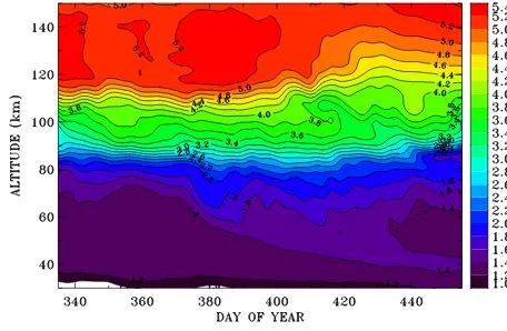
To put into perspective the CMAM-CIN NOXresults with respect to the observations by the ACE-FTS satellite exper-iment (Bernath et al., 2005), previously reported by Randall et al. (2009) and Manney et al. (2009), the model daily zon-ally averaged NOX VMRs were sampled in the ACE-FTS format (according to the latitude of the ACE-FTS daily so-lar occultations; see also Randall et al., 2009, their Fig. 1) for the three winter seasons of interest for days of year 1 to 90 from 1 January to 31 March, and are shown in Fig. 6. The ACE-FTS measurements are in the regime of solar oc-cultation and represent almost the same latitudes from year to year. The NOX log10 VMRs from 1 to 3 corresponding to 10 to 1000 ppbv are shown between 30 and 90 km height, to allow for direct comparison between the three winter sea-sons. The contour for NOX log10 VMR of 1.5 is used as a reference for the comparisons. The decrease of NOX VMR with increasing height around day 40 (10 February) is due to the change in direction of the ACE-FTS instrument obser-vation toward low latitudes, which is seen as a decrease in the NOXVMR. Around mid-February,∼day 40 (15 Febru-ary), the ACE-FTS continued observations at northern high latitudes and the observed NOXVMR increased.

In 2004 (Fig. 6a) the downward funnelling of NOX is first observed on about 25 January 2004 (day 25), when enhanced NOX reaches∼50 km height, but briefly receded back to 70 km before descending to 45 km for most of Febru-ary. The descent of the NOX is relatively weak and short-lived, and values of 1.5 log10 VMR (32 ppbv) dominate the lower mesosphere/upper stratosphere and were rapidly de-stroyed by vertical mixing at the upper boundary of the po-lar vortex and through photodissociation during popo-lar sun-rise in late February and early March. Most of the enhanced NOXremained in the UMLT region with perturbed isopleths above 80 km (Fig. 6a). The NOX(as the CO) mixing follow-ing the 2003/2004 SSW was correlated with the time of the cold stratopause (Fig. 1b). In 2004 ACE-FTS NOX observa-tions were available only after about day 50 (19 February) and showed high NOX VMR of about 200 ppbv (2.3 log10 VMR) reaching 50 km and lasting until the first half of March (e.g. Randall et al., 2009, Fig. 1), compared to modelled 32– 40 ppbv (1.5–1.6 log10 VMR) at the same altitude of 50 km, or a factor of∼5 smaller than the observations. This under-estimation can be, at least partially, explained by the miss-ing energetic particle precipitation production of NOXin the model simulations. This NOX enhancement continued into the stratosphere up until Northern Hemisphere equinox, de-creasing in magnitude to 50–20 ppbv (1.7–1.3 log10 VMR)

Figure 6. Evolution of the zonal mean NOX (NO + NO2) log10

VMRs in ppbv sampled in the ACE-FTS observing format as a function of day of year and altitude, from 1 January to 31 March (day 1–90) in (a) 2004, (b) 2006 and (c) 2009.

before being mixed and destroyed. This compares with 1.5– 1.4 log10VMR as simulated by the model (Fig. 6a).

very broad and intense, and although there was no further in-flux from above, high amounts of NOX(1.9–2.1 log10VMR or 79–125 ppbv) remained present in the lower mesosphere and upper stratosphere even during sunrise. The difference between the modelled and observed NOX in 2009 is of the order of 30–35 %.

Since the CMAM-CIN model does not account for EPP as the source of thermospheric NOX, the results shown in Fig. 6 give only the NOXresulting from meteorological conditions and dynamic perturbations associated with the nudging of the basic fields below 10 hPa (∼30 km). In spite of the model un-derestimation of the NOXVMR by 30–35 % particularly for 2006 and 2009 the model adequately represents the dynam-ics of the mesosphere and, since the latter is not vertically constrained, of the lower thermosphere above. This is also supported by available observations as discussed in Sect. 4.

Figure 7 shows the NOX vertical distribution from 30 to 150 km for the three winter seasons at 80◦_{N and day 335 to}

455 (1 December–31 March). Now that the dynamic effects on the NOX VMR have been confirmed in the stratosphere and mesosphere particularly in the comparison with the 2006 observations, the effect of the SSW on the UMLT region up to about 150 km and during the three SSW events is further examined. Once again, the picture outlined by the variations of the NOXVMR in Fig. 7 is that caused only by SSW dy-namical effects on the altitude region up to 150 km.

In the mesosphere there is a weak descent below 65 km, which in 2004 (Fig. 7a) reached down to 45 km with NOX log10VMR of 1.5 (32 ppbv), while the NOXlog10 VMR of 1.9 (79 ppbv) did not descend further than 70 km. In 2006 the NOX log10 VMR of 1.9 reached 65 km in late Febru-ary (Fig. 7b), while in 2009 (Fig. 7c) this level of VMR was maintained at 50 km well until mid-March. While the fun-nelling effect is observed mostly below 90 km in 2006 and 2009 (Fig. 7b, c), the atmosphere above appeared well mixed, except for downwelling of NOXat the time of the NOX de-scent (days 390–400, 25 January–5 February) and could be seen in the isopleths, which are decreasing in their height.

Another interesting difference between the state of the UMLT region in 2003/2004, on one hand, and that in 2005/2006 and 2008/2009 on the other is the fact that in the later case all isopleths with values between 2 and log10VMR (100–10 000 ppbv) were more or less horizontal and con-fined between 85 and 95 km height, while in 2003/2004 they were perturbed and expanded from 80 to 110 km. The lower thermosphere appeared compressed, with large NOX log10 VMR of 5.1 (126 ppmv) descending down to 120 km and even higher values of 5.3 (∼200 ppmv) from 120 to 140 km at the time of the beginning of NOXdescent around day 380 (15 January 2004). Such large NOXVMRs are observed only toward the end of March with the polar sunrise and at alti-tudes above ∼145–150 km, during the winters of 2006 and 2009. Further, while in 2005/2006 and 2008/2009 the VMR vertical gradient was steep and increased with height toward spring (end of March), in 2004 the period from mid-February

Figure 7. Evolution of the zonal mean NOX(NO + NO2, log10of

VMR in ppbv) at 80◦N for the altitude range from 30 to 150 km and from 1 December to 31 March (day 335–455) in (a) 2003/2004, (b) 2005/2006 and (c) 2008/2009.

to mid-March (day 410 to 440) indicated NOXlosses extend-ing to 130–140 km height.

602 M. G. Shepherd et al.: Stratospheric warming influence

February) with a decrease of the NOX VMR in the lower thermosphere, above ∼85–90 km (where the isopleths are almost flat) at the time when intense NOX mixing and loss take place in the lower mesosphere following the polar sun-rise (also Fig. 5a, b). The NOXappeared depleted, lifting the isopleths from the nominal altitude of∼120 km to 140 km. Above, the NOXfollows its seasonal variability with a maxi-mum around 160 km (not shown). In 2006 and 2009 (Fig. 7b and c) the picture is quite different. There is a large NOX gradient between 85 and 95–100 km, with almost horizon-tal isopleths indicating equilibrium between vertical mixing and horizontal transport with very small variation and almost no effect of polar sunrise and NOXloss above 110 km. Prior to the NOX downwelling around day 390–400 (26 January– 4 February 2006) there is a decrease of the NOXabove 90 km (to∼120 km), suggesting that in the lower thermosphere an upwelling was taking place carrying into the thermosphere air relatively poor of NOX compared to the ambient atmo-sphere. This is an extension of the same signature shown and discussed in Fig. 4 for CO and Fig. 5 for NOX. At 120 km the NOX VMR in 2006 was 10 times smaller than that in 2004 for the same period and altitude: only 12.6 ppmv (4.1 log10 VMR) in 2006 and 126 ppmv (5.1 log10VMR) in 2004. The 2009 SSW was the strongest among the three SSW events considered in terms of the magnitude of temperature change and wind shear. In the thermosphere there was a brief up-welling above∼100 km around days 383–385 (17–20 Jan-uary) at the time of the SSW followed by a massive NOX downwelling beginning around day 390 (25 January), which is seen to affect the NOX field up to at least 130 km, as is outlined by the isopleths of 4.3–4.5 log10VMR (Fig. 7c).

4 Discussion

Many authors have reported an enhancement of NOX in the mesosphere and stratosphere following the major strato-spheric warmings in January 2004, 2006 and 2009 (Man-ney et al., 2005, 2009; Randall et al., 2006, 2009; Degen-stein et al., 2005; Hauchecorne et al., 2007). Randall et al. (2009) showed that NOXincreased by a factor of 50 com-pared to winters without descent events. Siskind and Rus-sell (1996) and Siskind et al. (1997) investigated NO distri-bution up to 120 km from Halogen Occultation Experiment (HALOE)/UARS and showed that there was a transport of auroral NO into the upper stratosphere/mesosphere, which was interpreted as caused by the breaking of planetary waves at middle and low latitudes.

Natarajan et al. (2004) and Rinsland et al. (2005) sug-gested that a massive EPP event in October/November 2003 was responsible for the observed increase in NOXin the up-per stratosphere/mesosphere in January 2004, but Randall et al. (2005) argued that this EPP could not be responsible for the increased NOX observed in January in the upper strato-sphere/mesosphere because the SSW in December would

have led to the dilution of the EPP NOX with midlatitude air.

López-Puertas et al. (2005) (also Funke et al., 2007) anal-ysed MIPAS observations of NO2over the period of Octo-ber 2003 and April 2004 and concluded in agreement with Randall et al. (2005) that the observed enhancement in up-per stratospheric NO2in mid-January 2004 was most prob-ably caused by an unusually strong, compared to previous years, vortex and downward transport together with uncom-mon auroral activity over the entire winter 2003/2004 sea-son. Clilverd et al. (2007) were the first to provide iono-spheric evidence of thermoiono-spheric-to-stratoiono-spheric descent of polar NOX. They observed an enhanced descent of NOX in the mesosphere at 65–90 km starting on day 378 (13 Jan-uary 2004), a month before being seen in the stratosphere. Although there was a geomagnetic storm on day 387–388 (22–23 January 2004) GOMOS/Envisat observations indi-cated the storm did not create any observable effect on the NO2(and thus NOX)in the upper stratosphere/lower meso-sphere (50–70 km). However, the GOMOS data showed a significant amount of NO2below 70 km produced by a ge-omagnetic storm on day 407–408 (11–12 February 2004), which contributed to the body of NO2 descending into the stratosphere (Clilverd et al., 2007). This additional source of NOX is not captured in the CMAM-CIN model results shown in Figs. 5a and b and 7a since, as was already stated, the model does not account for the effect of EPP on the pro-duction of NOX. Clilverd et al. (2007) also concluded that the start date of the NOXdescent was not associated with any ge-omagnetic event, but that the formation of strong polar vor-tex giving rise to strong downward vertical transport from the pre-existing NOX thermospheric reservoir generated by LEPP (auroral low-energy particle precipitation, 1–10 keV) was more plausible.

conditions were fulfilled in 2003/2004, but not in 2005/2006 when no solar proton events or enhanced ionization were ob-served. This explains the very good agreement between the CMAM-CIN model results for 2006 shown in Fig. 5c and d and the ACE-FTS observations as reported by Randall et al. (2006). A similar argument applies to the CMAM-CIN 2009 results in Fig. 5e and f.

Most of the modelling of the vertical transport and the downward funnelling of the CO and NOX into the lower mesosphere and stratosphere has been concentrated on the al-titude range below 80–90 km using the European Centre for Medium-Range Weather Forecast (ECMWF) model nudged at 75–80 km height to the ACE-FTS observations (Salmi et al., 2011), the regular CMAM without nudging with a lid at 95 km (Jin et al., 2009), the NOGAPS-ALPHA4(Siskind et al., 2010) and recent versions of the CMAM-DAS (Data As-similation System) and the new CMAM20 relaxation scheme (Ren et al., 2011; McLandress et al., 2013).

Salmi et al. (2011) used the ECMWF and the Fin ROSE chemistry transport models to simulate the winter and strong descent of NOX and were able to produce a realistic NOX transport in the mesosphere while assuming NOX transport from above as observed by the ACE-FTS. The NOX model was constrained to time-dependent upper boundary condi-tions based on the ACE-FTS observacondi-tions between 75 and 85 km. The ECMWF was used up to 80 km, so the authors were able to study the NOX descent starting from the up-per mesosphere. However, since the upup-per boundary of the ECMWF was at 80 km it could not give any information on the dynamics and transport in the UMLT region. Ne-zlin et al. (2009) have shown that processes from the tropo-sphere and stratotropo-sphere can impact large-scale dynamics in the mesosphere, through upward-propagating resolved waves (Sankey et al., 2007) or through parameterized waves (Ren et al., 2008). Thus, since the SSW is forced by upward-propagating waves (Matsuno, 1971) the assimilation of ob-servations from the troposphere/stratosphere may be suffi-cient to describe the large-scale mesospheric response; thus, the CMAM-DAS (Ren et al., 2011) and the CMAM20 simu-lations (McLandress et al., 2013) were nudged below 1 hPa to SABER/TIMED observations and the ERA-Interim, respec-tively, with the latter using relaxation up to 1 hPa.

While experimental and model results have provided in-sight on the dynamic effects of SSW on the middle atmo-sphere and vertical transport in the stratoatmo-sphere/mesoatmo-sphere up to ∼100 km, the effect of SSW on the thermosphere is still not well known. A number of experimental results dur-ing the winter of 2008/2009 have shown perturbations in the neutral and ion temperature and winds (e.g. Goncharenko and Zhang, 2008; Conde and Nicholls, 2010; Funke et al., 2010; Kurihara et al., 2010), coinciding with the onset of the major stratospheric warming event of January and

4_{The Navy Operational Global Atmospheric Prediction System–}

Advanced Level Physics-High Altitude

February 2009. Therefore the modelling efforts have been extended into the upper atmosphere to examine the dynami-cal coupling between middle and upper atmosphere.

A model study by Liu and Roble (2002) employing the self-consistent TIME-GCM/CCM3 has examined the SSW impact on the MLT region, showing that at the time of SSW a warming of the lower thermosphere of the order of 20 K also occurs resulting from secondary downward circulation induced by equatorward mesospheric circulation. A similar warming of the lower thermosphere at the time of SSW is also produced by the CMAM-CIN. The CMAM-CIN ther-mospheric residual temperatures (Figs. 1 and 2), together with the zonal winds shown in Fig. 3, agree well with the re-sults of Liu and Roble (2002). In addition, the CMAM-CIN temperatures for the SSW in January 2009 at 80◦N agree well with the MIPAS temperature data averaged over 70– 90◦_{N during the same period both in structure and}

magni-tude, giving a warm residual temperature anomaly of 25 K with a peak at∼110 km and extending up to∼145 km with a value of 10 K around day 385–390 (20–25 January 2009) compared to the MIPAS residual temperatures of 15–20 K maximizing at∼120–130 km (Funke et al., 2010).

The whole atmosphere model GAIA has also been used to examine the atmospheric response to the 2009 major stratospheric warming from the ground to exobase. Liu et al. (2013) found that at northern high latitudes warming of 20 K occurs at all local times and altitudes of 110–130 km, in agreement with the seminal model study of Liu and Roble (2002) and the results presented herein. Further the GAIA simulations show a general cooling of the thermo-sphere global mean temperature above about 130 km extend-ing to as high as 400 km followextend-ing the onset of the SSW, which is also well seen in the CMAM-CIM results for the three SSWs (Figs. 1 and 2). These agreements give further support to the CMAM-CIN realistic representation of the ba-sic fields and dynamics of the UMLT region and its coupling with the atmosphere below.

604 M. G. Shepherd et al.: Stratospheric warming influence

the GW source at the lower boundary. Thus the choice of the non-orographic gravity wave drag (nGWD) parameterization considered, can lead to possible variability in the modelled atmosphere in the wave breaking altitudes (Liu and Roble, 2002).

Model simulations of a major SSW were also con-ducted employing the Whole Atmosphere Community Cli-mate Model v3.5 (WACCM; Kvissel et al., 2012) to exam-ine the transport of CO and ozone from the mesosphere into the stratosphere. The model was able to successfully repro-duce various characteristics of the middle atmosphere associ-ated with the SSW, including perturbations in the circulation and chemistry of the stratosphere and the mesosphere. This was the first detailed case study of SSW in a comprehensive free-running chemistry–climate model. Similar to the result herein it was shown that during the high-altitude stratopause reformation a mesospheric intrusion with high CO abun-dance unfolds and gets cut off from the atmosphere above, being surrounded by stratospheric air poor in CO. This CO funnel is further propagated downward and meridionally to midlatitudes over a period of 2–3 weeks before being com-pletely diluted in the ambient air.

The role of planetary and gravity waves was also examined with the WACCM for the same major SSW case by Limpa-suvan et al. (2012), who showed that the reversal of the zonal mean wind to westward at the time of the SSW onset leads to changes in the zonal-mean wave forcing. Following the SSW recovery planetary waves (both eastward and westward) were identified below the restored stratopause; eastward planetary waves can penetrate the restored stratopause, while no grav-ity waves were observed below it.

The CMAM-CIN simulations on the CO and NOX trans-port shown in Figs. 4 and 5 are consistent with the WACCM results reported by Kvissel et al. (2012). The study by Limpa-suvan et al. (2012) also gives support to the suggested possi-ble role of planetary waves penetrating through the restored stratopause and propagating throughout the mesosphere and into the lower thermosphere as the source of the dynamic perturbations seen in 2004 and Fig. 7a.

The CMAM-CIN used nudging to the ERAI only up to 10 hPa and was run free up to 200 km (for low solar ac-tivity) employing the Hines (1997) nGWD parameteriza-tion scheme. However, the agreement with other assimilaparameteriza-tion schemes both in magnitude and in the depiction of the height of the elevated stratopause and the polar vortex is found to be very good. As Siskind et al. (2010), Ren et al. (2011) and McLandress et al. (2013) have shown, nGWD is important in simulating the elevated stratopause following the SSW and for capturing the descent of mesospheric constituents. For example, Ren et al. (2011) have shown that the depiction of NOXdescent was sensitive to the use of nGWD and together with McLandress et al. (2013) demonstrated the importance of realistic depiction of gravity wave drag in the data assimi-lation schemes.

The results presented have shown that the CMAM-CIN is able to capture both the magnitude and the dynamics of the basic fields and the strong polar vortex during the three SSW below 90–100 km height. The model has also captured the evolution of the trace gases’ descent into the stratosphere following the SSWs and was found to be in good agreement with the ACE-FTS observations for 2006, when the observed downwelling was assigned to dynamics and the strong polar vortex. Since the model does not consider EPP, the predicted NOX in 2004, 2006 and 2009 should be considered as re-sulting only from dynamical transport and responding to the planetary and gravity waves propagating from below. In that regard the 2004 SSW shows the most dynamically perturbed mesosphere/lower thermosphere region from all three SSW events. The SSWs exert effects on the thermospheric neutral temperature at least up to 150 km, which amounts to∼50 to 60 K departures in temperature from its zonal mean values.

5 Summary and conclusions

The results presented have shown that the extended CMAM-CIN model is able to capture the magnitude and the dynam-ics of the vertical transport not only in the stratosphere and mesosphere, but also in the lower thermosphere (shown here up to 150 km), in part due to the more complete and extensive chemistry domain and physics representation used, which ex-tends across and well above the UMLT region. This enables a better representation of the upper atmospheric chemistry and NOXin particular.

The fact that, despite missing the EPP effects in this ver-sion of the CMAM, the model predictions for the January 2006 SSW were in such good agreement with the experimen-tal NOXand CO data in the mesosphere and stratosphere is consistent with the conclusion of Randall et al. (2009) that the observed funnelling of NOX into the stratosphere was more dynamically driven rather than due to EPP.

The extended CMAM-CIN simulations for 2003/2004, 2005/2006 and 2008/2009 appear to well represent the dy-namics of the MLT region and the coupling between the thermosphere and the stratosphere through the NOX and CO transport. The good agreement between the extended CMAM-CIN NOXwith the 2006 experimental data observed by ACE-FTS served to validate the model results and allowed examining the dynamical effects of stratospheric warmings on the upper mesosphere and lower thermosphere. Both CO and NOXexhibit a distinct latitudinal structure with the main descent close to the pole, which highlights the importance of the vortex re-establishment following the warming and the consequent funnelling of the upper atmosphere chemi-cal fields downward within the polar vortex. The descent in-creased close to the pole.

atmosphere and the lower thermosphere. Most operational analyses do not have sufficiently high-altitude model lids and associated local physics and chemistry to capture the meso-spheric response (Manney et al., 2008a), and only few of them include chemical fields simulated across and above the MLT region.

Acknowledgements. SRB and VIF would like to thank the Cana-dian Space Agency for support through the CMAM20 project.

Topical Editor C. Jacobi thanks two anonymous referees for their help in evaluating this paper.

References

Allen, D. R., Stanford, J. L., López-Valverde, M. A., Nakamura, N., Lary, D. J., Douglass, A. R., Cerniglia, M. C., Remedios, J. J., and Taylor, F. W.: Observations of middle atmosphere CO from the UARS ISAMS during the early northern winter 1991/1992, J. Atmos. Sci., 56, 563–583, 1999.

Allen, D. R., Stanford, J. L., Nakamura, N., López-Valverde, M. A., López-Puertas, M., Taylor, F. W., and Remedios, J. J.: Antarctic polar descent and planetary wave activity observed in ISAMS CO from April to July 1992, Geophys. Res. Lett., 27, 665–668, doi:10.1029/1999GL010888, 2000.

Allen, M., Yung, Y. L., Waters, J. W., Hack, W., Preuss, A. W., Wagner, H. G., and Hoyermann, K.: Vertical transport and photo-chemistry in the terrestrial mesosphere and lower thermosphere (50–120 km), J. Geophys. Res., 86, 3617–327, 1981.

Andrews, D. G., Holton, J. R., and Leovy, C. B.: Middle Atmo-sphere Dynamics, Acad. Press, 490 pp., 1987.

Barth, C. A.: Nitric Oxide in the Lower Thermosphere, Planet. Space Sci., 40, 315–336, 1992.

Barth, C. A., Bailey, S. M., and Solomon, S. C.: Solar-terrestrial coupling: Solar soft X-rays and thermospheric nitric oxide, Geo-phys. Res. Lett., 26, 1251–1254, 1999.

Barth, C. A., Mankoff, K. D., Bailey, S. M., and Solomon, S. C.: Global observations of nitric oxide in the thermosphere, J. Geo-phys. Res., 108, 1027, doi:10.1029/2002JA009458, 2003. Beagley, S. R., de Grandpre, J., Koshyk, J. N., McFarlane, N.

A., and Shepherd, T. G.: Radiative-dynamical climatology of the first-generation Canadian middle atmosphere model, Atmos. Ocean, 35, 293–331, 1997.

Beagley, S. R., McLandress, C., Fomichev, V. I., and Ward, W. E.: The extended Canadian middle atmosphere model, Geophys. Res. Lett., 27, 2529–2532, 2000.

Beagley, S. R., Boone, C. D., Fomichev, V. I., Jin, J. J., Semeniuk, K., McConnell, J. C., and Bernath, P. F.: First multi-year occul-tation observations of CO₂in the MLT by ACE satellite: obser-vations and analysis using the extended CMAM, Atmos. Chem. Phys., 10, 1133–1153, doi:10.5194/acp-10-1133-2010, 2010. Bernath, P. F., McElroy, C. T., Abrams, M. C., Boone, C. D., Butler,

M., Camy-Peyret, C., Carleer, M., Clerbaux, C., Coheur, P.-F., Colin, R., DeCola, P., DeMazière, M., Drummond, J. R., Dufour, D., Evans, W. F. J., Fast, H., Fussen, D., Gilbert, K., Jennings, D. E., Llewellyn, E. J., Lowe, R. P., Mahieu, E., McConnell, J. C., McHugh, M., McLeod, S. D., Michaud, R., Midwinter, C., Nas-sar, R., Nichitiu, F., Nowlan, C., Rinsland, C. P., Rochon, Y. J., Rowlands, N., Semeniuk, K., Simon, P., Skelton, R., Sloan, J. J.,

Soucy, M.-A., Strong, K., Tremblay, P., Turnbull, D., Walker, K. A., Walkty, I., Wardle, D. A., Wehrle, V., Zander, R., and Zou, J.: Atmospheric Chemistry Experiment (ACE), Mission overview, Geophys. Res. Lett., 32, L15S01, doi:10.1029/2005GL022386, 2005.

Bloom, S. C., Takacs, L. L., DaSilva, A. M., and Ledv-ina, D.: Data assimilation using incremental analysis up-dates, Mon. Weather Rev., 124, 1256–1271, doi:10.1175/1520-0493(1996)124<1256:DAUIAU>2.0.CO;2, 1996.

Brasseur, G. P. and Solomon, S.: Aeronomy of the middle atmo-sphere, Chemistry and Physics of the Stratosphere and Meso-sphere Series: Atmospheric and Oceanographic Sciences Li-brary, Vol. 32, Springer, 2005.

Conde, M. G. and Nicolls, M. J.: Thermospheric temperature above Poker Flat, Alaska, during the stratospheric warming event of January and February 2009, J. Geophys. Res., 115, D00N05, doi:10.1029/2010JD014280, 2010.

Cho, Y.-M. and Shepherd, G. G.: Correlation of airglow tem-perature and emission rate at Resolute Bay (74.68◦N), over four winters (2001–2005), Geophys. Res. Lett., 33, L06815, doi:10.1029/2005GL025298, 2006.

Clancy, R. T., Muhlemah, D. O., and Allen, M.: Seasonal variability of CO in the terrestrial mesosphere, J. Geophys. Res., 89, 9673– 9676, 1984.

Clerbaux, C., Coheur, P.-F., Hurtmans, D., Barret, B., Carleer, M., Colin, R., Semeniuk, K., McConnell, J. C., Boone, C., and Bernath, P.: Carbon monoxide distribution from the ACE-FTS solar occultation measurements, Geophys. Res. Lett., 32, L16S01 doi:10.1029/2005GL022394, 2005.

Clilverd, M. A., Seppälä, A., Rodger, C. J., Thomson, N. R., Licht-enberger, J., and Steinbach, P.: Temporal variability of the de-scent of high-altitude NOX inferred from ionospheric data, J.

Geophys. Res., 112, A09307, doi:10.1029/2006JA012085, 2007. Dee, D. P., Uppala, S. M., Simmons, A. J., Berrisford, P., Poli, P., Kobayashi, S., Andrae, U., Balmaseda, M. A., Balsamo, G., Bauer, P., Bechtold, P., Beljaars, A. C. M., van de Berg, L., Bid-lot, J., Bormann, N., Delsol, C., Dragani, R., Fuentes, M., Geer, A. J., Haimberger, L., Healy, S. B., Hersbach, H., Hólm, E. V., Isaksen, L., Kållberg, P., Köhler, M., Matricardi, M., McNally, A. P., Monge-Sanz, B. M., Morcrette, J.-J., Park, B. K., Peubey, C., de Rosnay, P., Tavolato, C., Thépaut, J.-N., and Vitart, F.: The ERA interim reanalysis: Configuration and performance of the data assimilation system, Q. J. Roy. Meteorol. Soc., 137, 553– 597, 2011.

Degenstein, D. A., Lloyd, N. D., Bourassa, A. E., Gattinger, R. L., and Llewellyn, E. J.: Observations of mesospheric ozone deple-tion during the October 28, 2003 solar proton event by OSIRIS, Geophys. Res. Lett., 32, L03S11, doi:10.1029/2004GL021521, 2005.

de Zafra, R. L. and Muscari, G.: CO as an important high-altitude tracer of dynamics in the polar stratosphere and mesosphere, J. Geophys. Res., 109, D06105, doi:10.1029/2003JD004099, 2004. Fomichev, V. I., Ward, W. E., Beagley, S. R., McLandress, C., Mc-Connell, J. C., McFarlane, N. A., and Shepherd, T. G.: Extended Canadian Middle Atmosphere Model: Zonal-mean climatology and physical parameterizations, J. Geophys. Res., 107, 4087, doi:10.1029/2001JD000479, 2002.