www.ann-geophys.net/32/83/2014/ doi:10.5194/angeo-32-83-2014
© Author(s) 2014. CC Attribution 3.0 License.
Annales
Geophysicae
Ion drift simulation of sudden appearance of sub-keV structured
ions in the inner magnetosphere
M. Yamauchi1, Y. Ebihara2, H. Nilsson1, and I. Dandouras3,4
1Swedish Institute of Space Physics (IRF), Box 812, 98128 Kiruna, Sweden 2Research Institute for Sustainable Humanosphere, Kyoto University, Uji, Japan
3CNRS, Institut de Recherche en Astrophysique et Planétologie (IRAP), BP 44346, 31028, Toulouse cedex 4, France 4University of Toulouse, UPS-OMP, IRAP, Toulouse, France
Correspondence to: M. Yamauchi ([email protected])
Received: 23 July 2013 – Revised: 13 November 2013 – Accepted: 9 January 2014 – Published: 12 February 2014
Abstract. Energy–latitude dispersed structured sub-keV ions in the inner magnetosphere often show significant develop-ment or intensification (by more than factor of 3) within 1–2 h near noon or afternoon where the azimuthal ion drift velocity at the sub-keV range is expected to be near zero. To examine whether such sudden appearances in the day-side can be explained by the drift motion of ions that are formed during substorm-related injections, we numerically simulated two such examples, one at noon and the other in the afternoon, based on the ion drift model. For both cases, the ion drift model with finite duration of proton source in the nightside can explain the observed large inbound–outbound differences in the sub-keV proton population without any new sources. Ion drift motion can thus cause rapid changes of complicated ion populations, at remote places from the source a long time after the substorm activities.
Keywords. Magnetospheric physics (energetic particles, trapped)
1 Introduction
Trapped hot ions at an energy range of 0.05–5 keV in the inner magnetosphere have complicated morphologies and mirror altitudes at different longitude, geomagnetic condi-tions, andLvalues (McIlwain, 1974; Quinn and McIlwain, 1979; Ejiri et al., 1980; Fennell et al., 1981; Sauvaud et al., 1981; Newell and Meng, 1986; Ebihara et al., 2001, 2004; Yamauchi et al., 1996, 2013). These trapped hot ions in the inner magnetosphere bounce between the Northern Hemisphere and the Southern Hemisphere with short bounce
periods of only about 11 min for 100 eV protons and 4 min for 1 keV protons atL=4 (see, e.g., Quinn and McIlwain, 1979). Therefore, the energy–latitude patterns of ion popula-tions of>100 eV in the inner magnetosphere are expected to be symmetric around the equator when the timescale is more than 0.5 h in this region.
Using this feature, Yamauchi et al. (2013) statistically ex-amined the temporal evolution of three types of structured ions that are commonly found at sub- to few keV range in the inner magnetosphere using inbound–outbound differ-ences in the proton data taken by the Cluster Ion Spectrom-etry (CIS) COmposition DIstribution Function (CODIF) in-strument (Rème et al., 2001). Cluster orbits of perigee traver-sals in the inner magnetosphere during the 2001–2006 period are nearly symmetric about the equatorial plane along nearly the same longitude, with less than 1–2 h local time (LT) dif-ference between the inbound and the outbound passes. The symmetry with respect to the equatorial plane for both the orbit and the motion of trapped ions allowed Yamauchi et al. (2013) to interpret the inbound–outbound differences in the latitudinal profile of the 0.1–1 keV ion population as tem-poral changes by, for example, ion energization, transport, or loss, with a timescale of the order of an hour.
traversals with significant enhancement (by more than fac-tor of 3 in energy flux density) or asymmetry in the energy– latitude dispersion direction are more frequently observed than the symmetric cases.
The second category is mostly found in the midnight sec-tor during subssec-torms, and sudden enhancement or appear-ance within 1 h is not surprising if the phenomenon is directly driven by the substorm (Yamauchi et al., 2013). The third cat-egory is found at all local times and can be interpreted as lo-cal phenomena with a short timeslo-cale of no more than 1 h. On the other hand, the first category (wedge-like dispersed ions) is often observed in the morning-to-noon sectors, and rep-resents the ion population that drifts more than a few hours after they are formed during substorms in the midnight-to-morning sectors (Ebihara et al., 2001; Yamauchi and Lundin, 2006; Yamauchi et al., 2009).
The inbound–outbound differences within 1–2 h for wedge-like dispersed ions can be understood if the observa-tion is in the morning sector, because the eastwardE×B drift exceeds the westward magnetic drift significantly at sub- to few keV range, such that ions may drift signifi-cantly within 1–2 h, whereEis the summation of co-rotation electric field and the externally imposed electric field. How-ever, the inbound–outbound differences in the noon and af-ternoon sectors cannot be intuitively understood because the azimuthal component of the ion drift at sub-keV energy is expected to be very small near noon and in the afternoon.
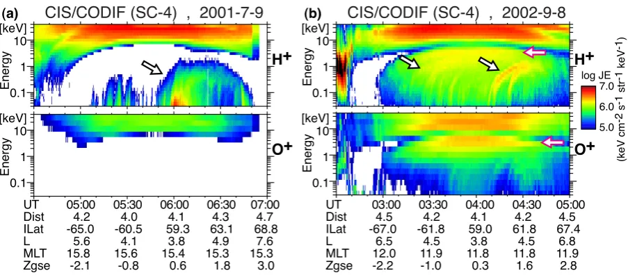
Figure 1 shows two such examples of wedge-like dis-persed ions observed by CODIF in spacecraft (SC) 4 during (a) 04:30–07:00 UT on 9 July 2001, and (b) 02:30–05:00 UT on 8 September 2002. The wedge-like dispersed ions are in-dicated by the black empty arrows. There are two types of asymmetry in this category: one with simple enhancement (or decay) in the intensity as shown in Fig. 1a (9 July 2001) and the other with asymmetric energy–latitude dispersion di-rections as shown in Fig. 1b (8 September 2002). Out of all clear events of the wedge-like dispersed ions observed during 2001–2006 by Cluster CIS/CODIF, the first type of asym-metry was observed 46 % of the time at 06–10 LT, 33 % of the time at 10–14 LT, and 35 % of the time at 14–18 LT re-spectively, and the second type of asymmetry was observed 30 % of the time at 06–10 LT, 23 % of the time at 10–14 LT, and 35 % of the time at 14–10 LT respectively (Yamauchi et al., 2013, Fig. 5).
The frequent occurrence of traversals with significant inbound–outbound differences in the wedge-like dispersed ions indicates either new injections or high eastward drift velocity even in the afternoon sector. For the drift velocity, Yamauchi and Lundin (2006) analyzed the Viking satellite data to show that the eastward ion drift could be much faster than the model, supporting the second possibility. However, a quantitative study such as the numerical simulation is needed to examine whether the drifting model alone can explain the enhancement within 1–2 h near local noon or if we need new sources to explain it (Yamauchi et al., 2013).
The purpose of this paper is to perform a particle drift simulation to answer this question. No past work simulated the wedge-like dispersed ions with inbound–outbound dif-ferences or asymmetries in the noon–afternoon sector. We use the same simulation model that was used in Yamauchi et al. (2009), which has successfully reproduced the ion pat-tern of an inbound–outbound symmetric event at 05 MLT ob-served by Cluster CIS/CODIF as a result of ion drift start-ing from low-energy (temperature is several tens of eV) ions at the nightside 8 Earth radii (RE) boundary. Two ex-amples shown in Fig. 1 are simulated: (a) SC-4 during 04:30–07:00 UT on 9 July 2001 and (b) SC-4 during 02:30– 05:00 UT on 8 September 2002. Since oxygen ions and pro-tons are different in Fig. 1, we simulate only propro-tons in this paper.
2 Simulation method
The numerical model used in Yamauchi et al. (2009) (orig-inally from Ebihara et al. (2001, 2008)) calculates the ion drift motion in the inner magnetosphere for both the energy-dependent magnetic (gradient-B and curvature) drift and the energy-independentE×Bdrift. The details of the numerical scheme are described in Ebihara et al. (2008). For magnetic and external electric fields, a dipole magnetic field and the Weimer-2001 type convection electric field model (Weimer, 2001) are employed with the solar wind parameters obtained from the 5 min resolution NASA/OMNI data set. Such a sim-ple magnetic field is sufficient for the present purpose be-cause we do not focus on the exact reconstruction of the source proton distribution. According to previous simulation works (e.g., Angelopoulos et al., 2002; Ebihara et al., 2004), the Weimer model gives a better explanation for the motion of ions in the inner magnetosphere than the Volland–Stern type model (Volland, 1973; Stern, 1975) does. For the parti-cle loss, we assumed charge exchange decay in the same way as Ebihara et al. (2001).
The actual calculation is performed in two steps: (a) we first trace the observed proton distribution backward using the phase-space mapping method (e.g., Kistler et al., 1999; Ebihara et al., 2008); (b) we then perform a forward drift sim-ulation assuming a boundary condition that is estimated from the back-tracing result. The backward tracing is necessary to estimate a proper boundary condition. Since one phase-space point in the observation is mapped to only one phase-space point by the Liouville theory, the backward tracing can cover only limited areas in location and energy for a given time.
UT Dist ILat L MLT Zgse
05:00 05:30 06:00 06:30 07:00 4.2 4.0 4.1 4.3 4.7 -65.0 -60.5 59.3 63.1 68.8 5.6 4.1 3.8 4.9 7.6 15.8 15.6 15.4 15.3 15.3 -2.1 -0.8 0.6 1.8 3.0
(keV cm
-2 s -1 str -1 keV -1)
H+
log JE 7.0 6.0 5.0
O+
UT Dist ILat L MLT Zgse
03:00 03:30 04:00 04:30 05:00 4.5 4.2 4.1 4.2 4.5 -67.0 -61.8 59.0 61.8 67.4 6.5 4.5 3.8 4.5 6.8 12.0 11.9 11.8 11.8 11.9 -2.2 -1.0 0.3 1.6 2.8
CIS/CODIF (SC-4) , 2002-9-8
[keV] 10 1 0.1 [keV] 10 1 0.1
CIS/CODIF (SC-4) , 2001-7-9
[keV] 10 1 0.1 [keV] 10 1 0.1
H+
O+
(a) (b)
Energy
Energy
Energy
[image:3.595.72.524.61.259.2]Energy
Fig. 1. Energy–time spectrograms of 4-pi averaged proton (H+, upper) and oxygen ion (O+, lower) differential energy fluxes observed by Cluster spacecraft-4 CIS/CODIF at 0.1–40 keV during (a) 04:50–07:00 UT on 9 July 2001, and (b) 02:30–05:00 UT on 8 September 2002. The black empty arrows indicate the energy–latitude dispersed structure sub-keV ions that are simulated in this paper, and red empty arrows indicate mono-energetic keV ions that are discussed in Yamauchi et al. (2009).
along the boundary for one time. The backward tracing is stopped when either protons reach the 8RE boundary or backward elapsed time exceeds a certain time (34 h in the present case).
For both examples in Fig. 1, the backward tracing result predicts a low-energy source distribution at 8RE boundary with proton density about 0.5 cm−3and proton temperature about 50 eV, and mainly in the nightside for a limited time interval. Such low-energy sources are already predicted in Ebihara et al. (2008) and Yamauchi et al. (2009), in which the simulations are compared with the observations. The pre-dicted low-energy proton distribution is also consistent with the cold ion supply from the ionosphere to the plasma sheet through the tail lobe (Engwall et al., 2009), in which the ion flow was obtained in the lobe region because of the low den-sity, but without solid information of exact temperature.
For the forward simulation, the reconstructed proton dis-tribution at 8RE is used as the boundary condition for both examples in Fig. 1. A limited time interval is mandatory to reproduce striping structure instead of filled structure in the spectrogram (Ebihara et al., 2001). The detailed scheme of the forward simulation including the assumed decay rate is described in Ebihara et al. (2004).
3 Numerical result
3.1 The 9 July 2001 event
The wedge-like dispersed ions (black empty ar-rows) in Fig. 1a are intensified more during the out-bound (05:50–06:50 UT) than during the inbound
(04:50–05:50 UT) at 15–16 MLT. Almost no signature is seen in the oxygen data for this signature, probably due to low counting rate of the oxygen ions. Figure 2 shows 5 min averaged OMNI solar wind parameters and auroral electrojet upper (AU) and lower (AL) indices for this event. The constant solar wind velocity (∼450 km s−1) and gradual change of the interplanetary magnetic field (IMF) northward component (fromBz∼ −5 nT to∼ +3 nT) during the past 10 h caused a monotonic drop of geomagnetic activity from its peak (AL∼ −700 nT) at around 02:30 UT to a quiet level (AL∼ −30 nT) after 06:10 UT.
Figure 3 shows the numerical simulation result of the pro-ton differential energy flux with local pitch angle of 90◦ at the location of observed latitude by the Cluster SC-4. The observed ions have pitch angles less than 90◦ in re-ality. However, the eastward drift velocities of the protons with smaller equatorial pitch angles than the observed ones are only slightly faster than the observed protons, even af-ter considering the difference in the drift velocity at different pitch angles for the competing magnetic drift (Ejiri, 1978; Yamauchi et al., 2006). It is possible to tune the pitch angle distribution to match the observation, but adding such a “free parameter” defocuses the most important mechanisms that cause the general asymmetric feature.
15 10 5 0 500 250 0 -250 -500 -750 15 10 5 0 -5 -10 -15 600 500 400 (a) (c) (b) (d) [n T ] [n T ] [km/ s] [cm -3]
[image:4.595.314.544.60.458.2] [image:4.595.52.284.64.368.2]17 18 19 20 21 22 23 0 1 2 3 4 5 6 7
IMF |B|
IMF BZ (GSM)
AL(11) AU(11) Solar wind speed Solar wind density
Solar Wind and AE(11) data , 8-9 July, 2001
UT
2001-07-08 2001-07-09
Fig. 2.
The solar wind OMNI data and geomagnetic indices from 11 AE stations on 8–9
July, 2001: (a) Solar wind density, (b) Solar wind velocity, (c) Interplanetary magnetic field
total strength (
|
B
|
) and northward component (B
z), and (d) AU and AL indices from 11
stations. All data are averaged over 5 min.
16
Fig. 2. The solar wind OMNI data and geomagnetic indices from 11 AE stations on 8–9 July, 2001: (a) solar wind density, (b) solar wind velocity, (c) interplanetary magnetic field total strength (|B|) and northward component (Bz), and (d) AU and AL indices from 11 stations. All data are averaged over 5 min.
we reduced the Weimer-2001 electric field by half in the day-side to reproduce the result shown in Fig. 3.
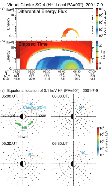
Figure 3a shows the virtual spectrogram using the simu-lated proton data assuming the Cluster SC-4 traversal. The simulation predicts the enhancement of the sub-keV popula-tion in a limited energy range during the outbound traversal only and not during the inbound. This asymmetry is similar to that shown in Fig. 1a. Figure 3b shows the elapsed time of observed protons from the start location that is located at 8RE on the nightside. The elapsed time is calculated from the backward particle tracing from the observed space–time, and, therefore, the figure contains even high-energy ions that are not simulated in the forward method. Because the convec-tion is time-varying, the calculated elapsed time is shorter for the enhanced sub-keV protons during the outbound (about 15 h) than for virtual sub-keV protons that would have ap-peared at the timing of inbound. In this way, the Cluster SC-4 traversed the inbound pass before the protons reached the satellite location. This is more clearly illustrated in Fig. 3c.
04:30 9.3 16.1 -45.8 05:00 5.6 15.8 -29.9 05:30 4.2 15.6 -11.5 06:00 4.1 15.4 7.8 06:30 5.3 15.3 26.0 07:00 8.5 15.3 42.1 UT L MLT MLAT 0 5 10 15 20 H o u rs
Virtual Cluster SC-4 (H+, Local PA=90°), 2001-7-9
(a) (b) [keV] 10 1 0.1 [keV] 10 1 0.1
Equatorial location of 0.1 keV H+ (PA=90°), 2001-7-9
Differential Energy Flux
(c) 103 104 105 106 107 # / cm
2 s
st r ke V 103 104 105 106 107 ke V / cm
2 s
st r ke V Elapsed Time En e rg y En e rg y
05:00 UT 06:00 UT
05:30 UT 06:30 UT
Cluster SC-4
midnight noon
dawn
drift
Fig. 3.
Simulated result for the first event on 9 July 2001. (a) Virtual spectrogram of Cluster
Spacecraft 4 using the simulated result. The format is the same as Fig. 1, i.e., except that
protons of local pitch angle of 90
◦are shown. (b) Elapsed time of ions that is obtained by the
backward tracing of the observed data. (c) Equatorial locations of the simulated stripes of
0.1 keV protons with 90
◦equatorial pitch angle, looking from the north every 30 min. The
spacecraft location is marked by the blue crosses
and ion drift direction for these 0.1 keV
protons is illustrated by solid blue arrows
. The finite length of red dots (0.1 keV protons)
comes from finite duration of proton injection at the source boundary in the nightside.
17
Fig. 3. Simulated result for the first event on 9 July 2001. (a) Virtual spectrogram of Cluster spacecraft-4 using the simulated result. The format is the same as Fig. 1 (i.e., except that protons of local pitch angle of 90◦are shown). (b) Elapsed time of ions that is obtained by the backward tracing of the observed data. (c) Equatorial loca-tions of the simulated stripes of 0.1 keV protons with 90◦equatorial pitch angle, looking from the north every 30 min. The spacecraft location is marked by the blue crosses, and ion drift direction for these 0.1 keV protons is illustrated by solid green arrows. The finite length of red dots (0.1 keV protons) comes from finite duration of proton injection at the source boundary in the nightside.
16 17 18 19 20 21 22 23 0 1 2 3 4 5 6 30 20 10 0 -10 -20 -30 1000 500 0 -500 -1000 -1500 -2000 (a) (c) (b) (d) 30 20 10 0 IMF |B|
IMF BZ (GSM)
AL(11) AU(11) Solar wind speed Solar wind density
UT 2002-09-08 2002-09-07 [n T ] [n T ] [km/ s] [cm -3] 600 500 400
Solar Wind and AE(11) data , 7-8 Sep., 2002
Fig. 4.
The same as Fig. 2 but for 7–8 September 2002.
18
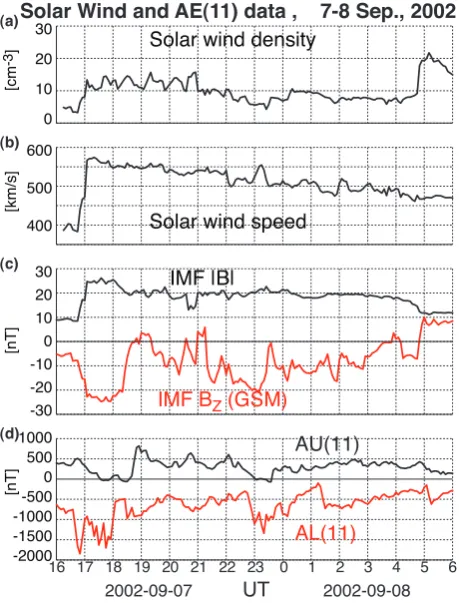
Fig. 4. The same as Fig. 2 but for 7–8 September 2002.
3.2 The 8 September 2002 event
A similar intensification of the wedge-like dispersed ions (black empty arrows) as the previous event is also found in Fig. 1b from the inbound (03:00–04:00 UT) to the out-bound (04:00–05:00 UT) at around local noon. In addition, the energy–latitude dispersion directions of the wedge-like dispersed ions are opposite (i.e., the same energy–time dis-persion direction) between the inbound and the outbound. Overlapping to these wedge-like dispersed ions, an intensi-fied ion band at around 1–3 keV is also observed as indicated by the red empty arrows. This ion band is outstanding in the oxygen data, and thus the O / H ratio is quite different be-tween the wedge-like dispersed ions and the ion band.
Figure 4 shows 5 min averaged OMNI solar wind param-eters and AU and AL indices for this event. After the coro-nal mass ejection (CME) hit the Earth at around 17:00 UT (about 11 h before the traversal), the solar wind veloc-ity gradually decreased from a high value of 550 km s−1 to about 480 km s−1 at the time of the Cluster traversal. During the same period, the IMF was very intense (about 20 nT total field) with a large southward component (Bz∼
−10 nT) from even before the CME arrival until just be-fore the Cluster traversal, causing very high geomagnetic ac-tivities of continuously AL<−500 nT with many substorm
02:30 11.3 12.2 -49.0 03:00 6.5 12.0 -34.4 03:30 4.6 11.9 -17.0 04:00 4.1 11.8 2.1 04:30 4.9 11.8 21.4 05:00 7.5 11.9 39.2 UT L MLT MLAT 0 1 2 3 4 5 6 H o u rs
Virtual Cluster SC-4 (H+, Local PA=90°), 2002-9-8
(a) (b) [keV] 10 1 0.1 [keV] 10 1 0.1 03:15 UT 03:45 UT 04:15 UT 04:45 UT Cluster SC-4 En e rg y Elapsed Time 103 104 105 106 107 ke V / cm
2 s
st r ke V (c) 103 104 105 106 107 # / cm
2 s
st
r
ke
V
Equatorial location of 0.1 keV H+ (PA=90°), 2002-9-8
En
e
rg
y
Differential Energy Flux
midnight
dawn
drift
Fig. 5.
The same as Fig. 3 but for the traversal on 8 September 2002.
19
Fig. 5. The same as Fig. 3 but for the traversal on 8 September 2002.
onsets, at around 16:40 UT, 18:30 UT, 22:50 UT, 01:20 UT and 05:10 UT.
Figure 5 shows the numerical simulation result in the same format as Fig. 3. For this simulation, protons are assumed to depart at the nightside outer boundary of 8REduring two in-tervals: 20:00–21:00 UT and 22:00–23:00 UT, with a density of 0.5 cm−3 and temperature of 50 eV, based on the back-ward tracing result of the observed protons. Figure 5a repro-duced two essential features of Fig. 1b: enhancement of the sub-keV ion population in the outbound, and the asymmet-ric energy–latitude dispersions with respect to the equator (increasing energy with time in both the inbound and out-bound).
dispersed ions and the band-like ions can be explained as different O / H ratios at different UTs at the outer bound-ary of 8RE. Since both the magnetic andE×B drifts are mass independent when comparing ions with the same en-ergy (Roederer, 1970, page 57; Yamauchi et al., 2006, Eq. 3), drift motion cannot filter out different ion species to explain the observed O / H difference.
Figure 5b also shows that the elapsed time for the out-bound sub-keV signature to reach the Cluster location is shorter than the virtual inbound sub-keV ions would have taken to reach the Cluster location. According to Fig. 5c, the last (westward-most) stripe of 0.1 keV proton has not reached the spacecraft location during the inbound traversal, while it passed the spacecraft location at the time of the outbound traversal. Thus, the spacecraft can observe significant devel-opment of the low-energy ion population within 1–2 h in this example too.
4 Discussion
We have simulated two examples at 15–16 MLT and 12 MLT, respectively, where the eastward ion drift normally slows down or even stagnates at the 0.1–1 keV energy range. The general features of the sub-keV ions are well reproduced even with the present simplified simulation settings, and the shape of the simulated wedge-like structure resembles those that are observed. In other words, the eastward drift is sufficiently fast to cause the inbound–outbound difference in the early afternoon sector when viewed by the Cluster satellite. Since the eastward drift is faster in the morning sector than the noon–afternoon sectors, we expect a higher degree of asymmetry there, as has previously been observed (Yamauchi et al., 2013).
During highly disturbed conditions, the induction electric field becomes dominant in the inner magnetosphere (e.g., Ohtani et al., 2010), and the modeling of the induction electric field is problematic. A stronger electric field than the ideal model field is also suggested from statistics of the wedge-like dispersed ions from Viking (Yamauchi and Lundin, 2006) and Cluster (Yamauchi et al., 2006). In such a case, the eastward drift velocity will be enhanced, mak-ing the energy–time and energy–latitude dispersions stronger (i.e., more curved in the spectrogram).
Here we assumed the source location (where ions do not have dispersion) at 8RE in the nightside, but the actual source location can be different, for example, in the late morning sector (Yamauchi et al., 2006) or even the near noon via direct supply from the ionosphere (Giang et al., 2009). Such an eastward shift of the source location shortens the eastward drift distance from the source to the spacecraft that traverses noon–afternoon sectors, making the elapsed time shorter and the energy–latitude dispersion weaker. Combin-ing the stronger electric field than the model and closer distance of the source location, the elapsed time can be
shortened while keeping the same strength of the energy– time dispersion. Therefore, the success of the present simu-lation with the 8REsource in the nightside does not neces-sarily exclude the possibility of other source locations.
Considering various source locations is particularly impor-tant in interpreting different populations. For example, in the second event (8 September 2002), the simulation reproduced the band-like ions at 1–3 keV as originating at a different start time than the sub-keV dispersed ions (Fig. 5b). This means that their source locations are not necessarily the same: the band-like keV ion may have traveled a longer distance (e.g., from the plasma sheet) than the sub-keV dispersed ions (e.g., from morning). The clear difference in the O / H ratio be-tween the two populations (Fig. 1b) supports this scenario.
There are many minor differences between the observa-tion and simulaobserva-tion if one compares them in detail. For ex-ample, the peak of the differential energy flux in the first event is found at much lower energy (30 eV) in the obser-vation (Fig. 1a) than in the simulation (about 300 eV). This indicates that the observed population can be a summation of two different sources: one the wedge-like dispersed ions that are simulated here, and the other the low-energy ion bursts (Yamauchi et al., 2013) that are also found in the inbound. Similarly, the peak flux problem is also seen in the inbound of the second event (1 keV in the observation in Fig. 1b and 200 eV in the simulation in Fig. 5a) and the central part (shape of peak differential energy flux is layer-like in Fig. 1b and rounded in Fig. 5a).
However, these details are rather a tuning problem using many realistic parameters, and such a discussion will miss the main point: the inbound–outbound differences and/or asymmetries of the sub-keV ions in the noon–afternoon sec-tor can be reproduced by drifting ions coming from the night-side. The modifications of the electric field or source location would not alter the main result of reproducing the inbound– outbound difference and/or asymmetry. One-hour difference can certainly mean a large change in the observation at a fixed magnetic local time. The exact timing and location that such an inbound–outbound difference can be observed in the virtual spacecraft depends on these external parameters. In the present case, we had to reduce the Weimer-2001 electric field by half to reproduce the observed spectrogram. This in turn provides a good test on the electric field model.
5 Conclusions
only. Furthermore, the second simulation also succeeded in reproducing the asymmetric energy–latitude dispersion of this population as well as band-like ions at around 1–3 keV. The simulation indicates that the eastward azimuthal ion drift is fast enough to make significant changes in the inner mag-netospheric sub-keV ion population within 1–2 h even in the noon–afternoon sector where the azimuthal ion drift is ex-pected to nearly stagnate.
Acknowledgements. The provisional AU/AL(11) indices are pro-vided by WDC-C2 for geomagnetism at Kyoto University. ACE level 2 (64 s averaged) data are provided by the ACE/MAG team and MAG/SWEPAM team through the ACE Science Center. The solar wind OMNI data are provided by NASA. The Cluster project is managed by the European Space Agency (ESA). The work is partly supported by the Swedish National Space Board (RS). Ya-mauchi thanks programs for disabled people in Sweden, which have made it possible for him to work.
Topical Editor C. Owen thanks C. Forsyth and one anonymous referee for their help in evaluating this paper.
References
Angelopoulos, V., Temerin, M., Roth, I., Mozer, F. S., Weimer, D., and Hairston, M. R.: Testing global storm-time electric field models using particle spectra on multiple spacecraft, J. Geophys. Res., 107, doi:10.1029/2001JA900174, 2002.
Ebihara, Y., Yamauchi, M., Nilsson, H., Lundin, R., and Ejiri, M.: Wedge-like dispersion of sub-keV ions in the dayside magneto-sphere: Particle simulation and Viking observation, J. Geophys. Res., 106, 29571–29584, 2001.
Ebihara, Y., Ejiri, M., Nilsson, H., Sandahl, I., Grande, M., Fen-nell, J. F., Roeder, J. L., Weimer, D. R., and Fritz, T. A.: Multiple discrete-energy ion features in the inner magneto-sphere: 9 February 1998, event, Ann. Geophys., 22, 1297–1304, doi:10.5194/angeo-22-1297-2004, 2004.
Ebihara, Y., Kistler, L. M., and Eliasson, L.: Imaging cold ions in the plasma sheet from the Equator-S satellite, Geophys. Res. Lett., 35, L15103, doi:10.1029/2008GL034357, 2008.
Ejiri, M.: Trajectory traces of charged particles in the magneto-sphere, J. Geophys. Res., 83, 4798–4810, 1978.
Ejiri, M., Hoffman, R. A., and Smith, P. H.: Energetic particle pene-tration into the inner magnetosphere, J. Geophys. Res., 85, 653– 663, 1980.
Engwall, E., Eriksson, A. I., Cully, C. M., André, M., Torbert, R., and Vaith, T.: Earth’s ionospheric outflow dominated by hidden cold plasma, Nat. Geosci., 2, 24–27, doi:10.1038/ngeo387, 2009. Fennell, J. F., Croley Jr., D. R., and Kaye, S. M.: Low-energy ion pitch angle distributions in the outer magnetosphere: Ion zipper distributions, J. Geophys. Res., 86, 3375–3382, doi:10.1029/JA086iA05p03375, 1981.
Giang, T. T., Hamrin, M., Yamauchi, M., Lundin, R., Nilsson, H., Ebihara, Y., Rème, H., Dandouras, I., Vallat, C., Bavassano-Cattaneo, M. B., Klecker, B., Korth, A., Kistler, L. M., and McCarthy, M.: Outflowing protons and heavy ions as a source for the sub-keV ring current, Ann. Geophys., 27, 839–849, doi:10.5194/angeo-27-839-2009, 2009.
Kistler, L. M., Klecker, B., Jordanova, V. K., Möbius, E., Popecki, M. A., Patel, D., Sauvaud, J. A., Rème, H., Di Lellis, A. M., Korth, A., McCarthy, M., Cerulli, R., Bavassano Cattaneo, M. B., Eliasson, L., Carlson, C. W., Parks, G. K., Paschmann, G., Baumjohann, W., and Haerendel, G.: Testing electric field mod-els using ring current ion energy spectra from the Equator-S ion composition (ESIC) instrument, Ann. Geophys., 17, 1611–1621, doi:10.1007/s00585-999-1611-2, 1999.
McIlwain, C. E.: Substorm injection boundaries, in: Magneto-spheric Physics, edited by: McCormac, B. M., 143–154, D. Rei-del, Hingham, Mass, 1974.
Newell, P. T. and Meng, C. I.: Substorm introduction of 1 keV mag-netospheric ions into the inner plasmasphere, J. Geophys. Res., 91, 11133–11145, 1986.
Ohtani, S., Korth, H., Keika, K., Zheng, Y., Brandt, P. C., and Mende, S. B.: Inductive electric fields in the inner magnetosphere during geomagnetically active periods, J. Geophys. Res., 115, A00I14, doi:10.1029/2010JA015745, 2010.
Quinn, J. M. and McIlwain, C. E.: Bouncing ion clusters in the Earth’s magnetosphere, J. Geophys. Res., 84, 7365–7370, 1979. Réme, H., Aoustin, C., Bosqued, J. M., Dandouras, I., Lavraud, B., Sauvaud, J. A., Barthe, A., Bouyssou, J., Camus, Th., Coeur-Joly, O., Cros, A., Cuvilo, J., Ducay, F., Garbarowitz, Y., Medale, J. L., Penou, E., Perrier, H., Romefort, D., Rouzaud, J., Vallat, C., Alcaydé, D., Jacquey, C., Mazelle, C., d’Uston, C., Möbius, E., Kistler, L. M., Crocker, K., Granoff, M., Mouikis, C., Popecki, M., Vosbury, M., Klecker, B., Hovestadt, D., Kucharek, H., Kuenneth, E., Paschmann, G., Scholer, M., Sckopke, N., Seiden-schwang, E., Carlson, C. W., Curtis, D. W., Ingraham, C., Lin, R. P., McFadden, J. P., Parks, G. K., Phan, T., Formisano, V., Amata, E., Bavassano-Cattaneo, M. B., Baldetti, P., Bruno, R., Chion-chio, G., Di Lellis, A., Marcucci, M. F., Pallocchia, G., Korth, A., Daly, P. W., Graeve, B., Rosenbauer, H., Vasyliunas, V., Mc-Carthy, M., Wilber, M., Eliasson, L., Lundin, R., Olsen, S., Shel-ley, E. G., Fuselier, S., Ghielmetti, A. G., Lennartsson, W., Es-coubet, C. P., Balsiger, H., Friedel, R., Cao, J.-B., Kovrazhkin, R. A., Papamastorakis, I., Pellat, R., Scudder, J., and Sonnerup, B.: First multispacecraft ion measurements in and near the Earth’s magnetosphere with the identical Cluster ion spectrometry (CIS) experiment, Ann. Geophys., 19, 1303–1354, doi:10.5194/angeo-19-1303-2001, 2001.
Roederer, J. G.: Dynamics of Geomagnetically Trapped Radiation, Springer-Verlag, New York, 1070, 1970.
Sauvaud, J.-A., Crasnier, J., Mouala, K., Kovrazhkin, R. A., and Jor-jio, N. V.: Morning sector ion precipitation following substorm injections, J. Geophys. Res., 86, 3430–3438, 1981.
Stern, D. P.: The motion of a proton in the equatorial magneto-sphere, J. Geophys. Res., 80, 595–599, 1975.
Volland, H.: A semiempirical model of large-scale magnetospheric electric fields, J. Geophys. Res., 78, 171–180, 1973.
Weimer, D.: An improved model of ionospheric electric poten-tials including substorm perturbations and application to the Geospace Environment Modeling November 24, 1996, event, J. Geophys. Res., 106, 407–416, 2001.
Yamauchi, M., Lundin, R., Eliasson, L., and Norberg, O.: Meso-scale structures of radiation belt/ring current detected by low-energy ions, Adv. Space Res., 17, 171–174, 1996.
Yamauchi, M., Brandt, P. C., Ebihara, Y., Dandouras, I., Nilsson, H., Lundin, R., Rème, H., Vallat, C., Lindquvist, P.-A., Balogh, A., and Daly, P. W.: Source location of the wedge-like dispersed ring current in the morning sector during a substorm, J. Geophys. Res., 111, A11S09, doi:10.1029/2006JA011621, 2006.
Yamauchi, M., Ebihara, Y., Dandouras, I., and Rème, H.: Dual source populations of substorm-associated ring current ions, Ann. Geophys., 27, 1431–1438, doi:10.5194/angeo-27-1431-2009, 2009.