DOI 10.1007/s11242-008-9286-9
An Apparent Interface Location as a Tool to Solve
the Porous Interface Flow Problem
Tomer Duman · Uri Shavit
Received: 14 January 2008 / Accepted: 20 August 2008 / Published online: 30 September 2008 © Springer Science+Business Media B.V. 2008
Abstract A new approach for solving the laminar flow problem above a porous medium is presented here, using an apparent interface for which both superficial velocity and intrinsic shear stress are continuous. The derivation of this approach is based on a detailed investigation of the Ochoa-Tapia and Whitaker (Int. J. Heat Mass Transfer 38:2635–2646, 1995a) jump condition and its sensitivity to the value ofβ(the jump condition coefficient) and to an error in the interface location. While the value of the jump condition coefficient is highly sensitive to the interface location, the new apparent interface approach does not require an a priori information about the location of the interface. This approach can be easily used knowing only one measurable parameter—the maximum velocity or the flow rate. Validation of the apparent interface approach against measurements from other works shows that it can be successfully used to predict the velocity profile for different geometrical models.
Keywords Beavers and Joseph boundary condition·Brinkman equation·Jump condition· Apparent interface location
1 Introduction
The phenomenon of flow above porous domains can be found in a variety of natural environ-ments as well as in a long list of industrial applications. Such flow problems include overland flow during rainfall events, wetland flows, filtering, cooling, and processing flows in the elec-trical, chemical, and food industries. Other examples that were addressed in the literature are sea water flow above coral reefs (Lowe et al. 2008) and air flow above constructed areas (Finnigan 2000). In all of these cases, knowledge of the flow field within and above the inter-face is important as it allows the modeling of associated mass and heat transport problems
T. Duman·U. Shavit (
B
)Civil and Environmental Engineering, Technion, Haifa 32000, Israel e-mail: [email protected]
T. Duman
and a better understanding of biological and ecological processes. Although this subject has been investigated in the last few decades, a satisfactory solution has not been found.
The description of the flow at the fluid-porous interface can be obtained either microscopically or macroscopically. A microscopic description of such a problem can be achieved numerically by solving the governing Navier–Stokes equations which are valid in the entire fluid domain. The advantage of the microscopic description lies in the ability to map the exact velocity in space (as opposed to the average velocity in the macroscopic description), but the Navier–Stokes equations, being microscopic, require the knowledge of the detailed flow domain geometry, which cannot be achieved for most practical applications. Even for known geometries, computing time is still too long even for the most advanced computers available today. As of today, the few studies that have provided microscopic computations were limited to simple geometries (e.g.,Breugem and Boersma 2005;Rosenzweig and Shavit 2007).
To overcome this problem, two macroscopic approaches are available: the “single-domain approach” and the “two-domain approach.” In the single-domain approach the system is treated as a continuum and the same equations are being solved in the entire domain. The transition from the free fluid to the porous region is achieved through specifying the spatial variation of properties such as permeability, apparent viscosity, and porosity. In the two-domain approach, the system is composed of two different homogenous regions, the porous domain and the free flow domain, which are coupled at the interface. The flow in the two domains is formulated using different equations and an internal boundary condition which is needed to solve for potential discontinuity in the intrinsic velocity gradient at the interface.
As of today, most studies treated the momentum transfer across the interface by using the two-domain approach (e.g.,Beavers and Joseph 1967;Breugem et al. 2005;Chandesris and Jamet 2006,2007;Goyeau et al. 2003;Neale and Nader 1974;Ochoa-Tapia and Whitaker 1995,b). First attempt was made byBeavers and Joseph(1967) (BJ for short), who applied a semi-empirical slip boundary condition for the velocity at the interface to couple Stokes and Darcy equations:
du
dy
y=0+
= √α
k(ui−UD) (1)
where y= 0+ denotes the interface location on the free flow side, k is the permeability of the porous domain,UD is the Darcy velocity inside the porous domain,ui is the free
fluid velocity at the interface, andα is an empirical dimensionless slip coefficient, which typically varies between 0.1 and 4. Studies have shown that the value ofαis sensitive to the interface geometry (Richardson 1971;Taylor 1971) and its exact location (Larson and Higdon 1986,1987;Saffman 1971;Sahraoui and Kaviany 1992;Saleh et al. 1993). This last finding indicates that without information about the exact location of the interface, Eq. 1cannot be used and the flow problem cannot be solved.
While the original analysis of BJ was limited to the free flow domain, others (e.g.Neale and Nader 1974) included in their analysis the flow inside the porous domain which is often modeled by the Darcy–Brinkman equation:
µeff
d2u
dy2 −
µ
k u =
dpf
dx (2)
whereuis the superficial average velocity,pfis the intrinsic average pressure,µis the
fluid dynamic viscosity, andµeff denotes the effective viscosity of the fluid in the porous
from the molecular viscosity of the fluid (Shavit et al. 2002). While continuity at the interface is typically ignored by the BJ approach, many studies that used Eq.2assumed continuity in both the superficial velocity and the effective stress. This continuity is easily achieved since the Darcy–Brinkman equation (Eq.2) and the Stokes equation are of the same order. However, the continuity of stress at the interface is not necessarily valid for the average macroscopic stress (Nield 1991). Note that when different macroscopic stresses are applied on the two sides of the interface, an exact location of the interface must be given.
It will be shown later that planar averaging of the microscopic solution exhibits a contin-uous shear stress within the fluid phase and within the porous phase. This continuity breaks down when moving from the fluid to the porous domain across a sharp interface, due to a momentum transfer to the solid phase which occurs below the interface but absent above it. A promising approach was developed byOchoa-Tapia and Whitaker(1995,b) (OTW for short) who, using the method of volume averaging, derived a boundary condition using a jump in the effective shear stress, instead of continuity, to couple the Stokes and Darcy– Brinkman equations at the interface,
µeff
du
dy
y=0−
−µdu dy
y=0+
=β√µ
k u|y=0 (3)
whereβis an adjustable jump coefficient which is empirically determined. The OTW jump condition has a more convincing physical meaning and produces better results when compared with the BJ’s slip condition. As will be discussed later, we note that OTW have usedµeff=
µ/φin the original form of Eq.3. It was found that a good agreement is achieved when β ∼1.α, on the other hand varies over a factor of 40 (Breugem et al. 2005). Many of the recent studies used the jump condition to solve interface flow problems: Breugem et al. 2005;Kuznetsov and Xiong 2003;Silva and de Lemos 2003a,b; to list a few. Other recent studies focused on the attempt to predict the value ofβ(Ochoa-Tapia and Whitaker 1995b; Chandesris and Jamet 2006;Goyeau et al. 2003;Valdes-Parada et al. 2007).
As was the case with the BJ condition and with the Darcy–Brinkman equation, the two-domain approach can be solved only if the exact location of the interface is known a priori. However, an exact determination of the interfacial position is difficult or even impossible to obtain. Therefore, when the interface location is unknown neither of the above formulations can be used. The objective of the current paper is to explore first a case study of the interface problem (used byTaylor 1971) in order to examine the sensitivity of the jump condition model to the accurate determination of the interface location, and then to develop an alternative prediction tool that is based on an apparent interface location with zero stress jump at the interface.
x
u(y)
F
u
lly De
v
eloped Laminar Flo
w
Free Flow Domain
Porous
Medium
y
(a) (b)
h
z
L
d
Apparent interface
0 ξ
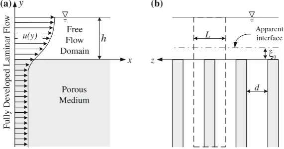
Fig. 1 Flow geometry.aSide view and the schematic velocity profile near a permeable interface. Flow is unidirectional in thex-axis direction.bFront view of the Taylor brush configuration. A repeating elementary unit is marked with a dashed line
2 Macroscopic Governing Equations
We consider a laminar unidirectional free flow over a porous surface. In the “two-domain approach” the system is separated into two different homogenous regions with an interface at
y=0 (Fig.1a). We use the distinction between the superficial and intrinsic volume averages, where the superficial average of propertyψis defined by
ψ = 1
V
Vf
ψdV (4)
and the intrinsic average is
ψf=
1
Vf
Vf
ψdV (5)
whereVf denotes the fluid phase volume within the averaging volumeV. The relationship
between these two averages is given by
ψ =φψf, φ=Vf/V (6)
whereφis the porosity. In the free flow domain (y≥0), the velocity is solved by the Stokes equation:
−dPf
dx +µ
d2u
dy2 =0, (7)
while in the porous domain (y≤0), the flow is modeled by the Darcy–Brinkman equation
(Eq.2). The boundary conditions for the specified problem include a stress jump condition (Eq.3) at the interface, zero shear at the top free boundary (y=h),
du
dy
y=h
=0 (8)
and Darcy velocity deep inside the porous medium (y→ −∞),
u|y→−∞= −k
µ dpf
[image:4.439.77.363.59.209.2]3 The Taylor Brush Configuration
3.1 Geometry
The geometrical configuration as was used byTaylor(1971) is shown in Fig.1b. It consists of an infinite number of walls divided by grooves, where the fluid flow is in thexdirection within and above the grooves. The walls and grooves are made of a uniform thickness and a depth which is considered infinite. The model porosity is defined by:
φ=d/L (10)
wheredandLare the width of the groove and the repeating elementary unit, respectively (see Fig.1b). The permeability,k, can be computed using the Poiseuille solution for flow between two parallel flat plates:
k=d3/12L=φ3L2/12 (11)
Equation11shows that for every combination ofφandk, only one positive value ofL
is valid. Thus, the model can produce a porous medium with any desirable combination of permeability and porosity using a uniform thickness for both walls and grooves. Hence, the porosity and permeability of the current configuration are the only parameters needed to fully describe the porous medium.
3.2 Microscopic Flow Solution
Numerical solutions of the microscopic equations (2D Stokes equation in the fluid phase) for the 2D brush configuration were obtained using Comsol Multiphysics, a finite element analysis and solver software package. Using the symmetric nature of the brush, equations were solved for only one half of the repeating unit, containing one half of a wall and one half of a groove. Different combinations ofdandLwere examined for porosity values between 0.3 and 0.9 and for permeability values between 5×10⁻⁴and 2×10⁻²cm2(covering approximately
800 combinations). The fluid density, viscosity, and pressure gradient were specified asρ= 1 g cm−3,µ=0.01 g cm−1s−1, and dPf/dx= −0.01 g cm−2s−2, respectively. Solutions
were examined for water depthhof 1 and 2 cm above the nominal interface. The nominal interface location is defined at the top of the walls and serves as the origin of they-axis, as shown in Fig.1b. Boundary conditions were no-slip on the solid surfaces, symmetry condition on the side boundaries and zero shear at the top and bottom. The fluid domain was meshed with quadratic-Lagrange elements. Mesh was refined until further refinement did not change the maximum velocity of the 2D fluid domain solution by more than a relative ratio of 0.0001.
3.3 Macroscopic Flow Solution
The solution of the 1D Stokes equation (Eq.7) for the free fluid region (y ≥0)using zero shear for the top boundary condition (Eq.8) and a known slip velocity at the interface is
u(y)= 1
2µ dpf
dx y 2− 1
µ dpf
dx h·y+ u|y=0, 0≤y≤h (12)
To solve the yet unknown average velocity at the interface (aty=0), an assumption needs to be made for the value of the effective viscosity,µeff. Different expressions forµeff can
bydu Plessis and Masliyah(1988), who used the same expression. Later,Whitaker(1999, p. 173) derived the Brinkman correction to Darcy’s law using a volume averaging procedure and also reached the same expression. He claimed that the use of an empirical effective viscosity term in the Brinkman equation is a result of a confusion between the intrinsic and the superficial velocities, which are distinguished by a factor ofφ. We therefore choose to follow this formulation and use hereµeff =µ/φ. As a result, the shear stresses in the OTW
jump condition (Eq.3) become the intrinsic stresses. The solution of the Darcy–Brinkman equation (Eq.2) in the porous domain (y≤0)givenµeff=µ/φand using the Darcy velocity
for the bottom boundary condition (Eq.9,y= −∞)is
u(y)=C·ey√φ/k− k
µ dpf
dx , −∞ ≤ y≤0 (13)
Thus, the velocity and the velocity gradients at the interface are
u|y=0=C− k
µ dpf
dx ;
du
dy
y=0+
= −h µ
dpf
dx ; (14)
du
dy
y=0−
=
φ
k ·C
Substituting (14) into the momentum jump condition (Eq.3) yields
C = −kλ
µ dpf
dx (15)
whereλis nondimensional and defined by:λ= h/
√
k+β 1/√φ−β.
3.4 Comparing the Microscopic with the Macroscopic Solutions
A comparison between the macroscopic model and the microscopic solution is based on averaging the microscopic flow field while using a representative elementary volume (REV). Since the Taylor brush configuration is periodic in the lateral direction (thez- axis), the REV size in that direction is defined as the width of the repeating elementary unit,L. Since the brush configuration is not changing along they-axis direction inside the porous medium, there are no restrictions on the choice of the REV height and any given value can be used. However, to observe the stress jump the REV height at the interface region has to be as small as possible. Therefore, the macroscopic flow was obtained by a planar averaging of the microscopic solution. This was obtained by averaging the velocity field along thex–z(horizontal) plain. The generated one-dimensional velocity profile was then compared with the macroscopic analytical solution using the jump condition, as shown in the following section.
4 Jump Condition
4.1 Investigating the Jump Condition Solution
velocity field and defineUmaxas the maximum velocity which is typically obtained aty=h.
The microscopic solution is considered as the ‘true’ velocity, and thereforeUmaxis named
the ‘true’ maximum velocity. The analytical solution of the macroscopic flow (Eqs.12–15) was then compared with the averaged microscopic (‘true’) solution by adjustingβsuch that the maximum velocity of the macroscopic solution u|y=his equal toUmax. The values of
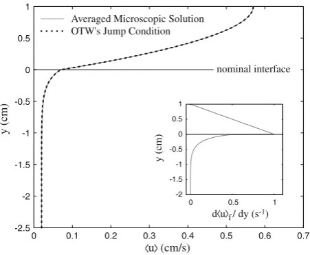
βthat were obtained in the fitting process varied between−0.41 and−1.33. The maximum velocity was chosen as a fitting test since the largest deviation is reached at the top boundary. Such a fitting test is especially adequate since the more common no-slip condition at the top boundary (e.g.,Beavers and Joseph 1967;Taylor 1971) was replaced by a no-shear condition. As will be shown later, a comparison of the interface velocity is problematic in the case of the two-domain approach since a good fit between the two profiles can be achieved with different interface velocities by moving the interface location. Figure2demonstrates a comparison between the superficial velocity profiles obtained from both the planar averaged microscopic solution and the OTW jump condition for a porosity of 0.5 and a permeability of 0.02 cm2. The figure subset shows the intrinsic derivative of the averaged microscopic solution, which represents the shear stress in the fluid. Figure2shows that the planar averaged microscopic velocity profile is continuous at the interface, but a jump occurs in the intrinsic shear stress, providing a clear physical justification for the OTW’s jump condition. Figure2demonstrates that a correct choice ofβprovides an excellent agreement between the averaged microscopic solution and the analytical OTW solution along the two homogenous domains and inside the transition zone. Note that the value ofβcalculated for all the investigated configurations was always negative. The physical meaning is that the shear stress shows a sudden decrease when entering the porous domain.
4.2 Sensitivity of the Jump Condition to the Interface Location
To examine the influence of the interface location on the velocity solution, we introduce a parameterξwhich is defined as the deviation from the nominal interface in they-axis positive
0 0.1 0.2 0.3 0.4 0.5 0.6 0.7
-2.5 -2 -1.5 -1 -0.5 0 0.5 1
<
u>
(cm/s)y (cm)
Averaged Microscopic Solution OTW's Jump Condition
nominal interface
f
0 0.5 1
-2 -1.5 -1 -0.5 0 0.5 1
d
<
u>
/dy (s-1)y (cm)
[image:7.439.108.334.401.586.2]direction.ξ can be regarded as an error in specifying the interface location. The effect of such an error can be calculated analytically by substitutingξ into the analytical solution of the macroscopic equations (Eqs.12–15). The maximum velocity, which serves as our fitting test, as a function ofξis expressed as follows:
u|y=h= −
1 2µ
∂pf
∂x
ξ2−2
h+
√
k
1/√φ−β
ξ+h2+2k(λ+1) (16)
Equation16shows that the maximum velocity function is parabolic with respect toξ. For small displacementsu(ξ)|y=his approximately linear. It can also be shown that the porous medium parameters have a small effect on the velocity. Thus, using an order of magnitude analysis (see Appendix A) the deviation from the actual maximum velocity,Umax, can be
expressed as:
Umax− u|y=h≈ −
1 µ
∂pf
∂x hξ (17)
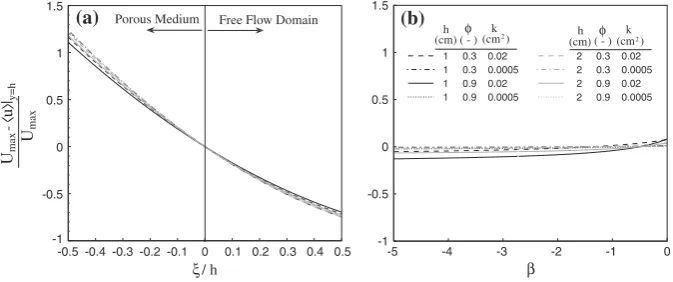
In Eq.17the change in the maximum velocity is a linear function ofξand does not depend on the porosity or the permeability. Indeed simulations presented in Fig.3a show a similar, approximately linear, behavior of the relative change in maximum velocity with respect to the relative change in the interface location (ξ/h) for all combinations of porosity and permeability. While this result is obvious from the analytical expression in Eq.17, the behavior of the maximum velocity as a function ofβis more complicated to find analytically. Figure3b presents simulation results for the change in the maximum velocity versusβwhile keeping the interface location at its nominal position (ξ =0). A comparison between Fig.3a and b shows that the solution is by far more sensitive to the interface positionξthan to the value ofβ. This result indicates that the OTW’s jump condition can provide a good prediction only if the interface location is specified with no error or uncertainty. When the interface location is determined with even a small error, a very large prediction mistake is generated by the OTW’s jump condition model. This mistake will be hard to correct by readjusting the value ofβ, due to its low effect on the calculated velocity. Furthermore, the values ofξ/h that generate a velocity error of tens of percents are often too small to be measured in practice.
As was shown in Fig.2, the OTW’s jump condition provides an excellent prediction. Figure3, however, shows that a small error in the interface location results in large prediction
-5 -4 -3 -2 -1 0
-1 -0.5 0 0.5 1 1.5
β 1 0.3 0.02 1 0.3 0.0005 1 0.9 0.02 1 0.9 0.0005
2 0.3 0.02 2 0.3 0.0005 2 0.9 0.02 2 0.9 0.0005 ( - )
(cm)h φ (cmk2)
-0.5 -0.4 -0.3 -0.2 -0.1 0 0.1 0.2 0.3 0.4 0.5 -1
-0.5 0 0.5 1 1.5
ξ/ h
Porous Medium Free Flow Domain
Umax -
<
u>
|y=h
Umax
( - ) (cm)h φ (cm2)
k
(a) (b)
Fig. 3 The change of the maximum macroscopic velocity u|y=h relative toUmax, as a function of the
[image:8.439.54.391.451.592.2]0 0.1 0.2 0.3 0.4 0.5 0.6 0.7 -2.5
-2 -1.5 -1 -0.5 0 0.5 1
<
u>
(cm/s)y (cm) Averaged
Microscopic Solution
OTW ξ = - 0.02 cm β = -2.06 OTW ξ = 0 cm β = -1.02 OTW ξ = 0.046 cm β = 0 OTW ξ = - 0.02 cm β = -1.02
0.05 0.1 0.15 -0.8
-0.6 -0.4 -0.2 0 0.2
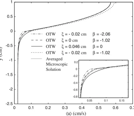
Fig. 4 Velocity profiles obtained with the OTW jump condition for several interface locations, with the value ofβreadjusted to fit the maximum value of the averaged microscopic solution. The velocity profile near the interface is magnified in the figure subset.φ=0.5,k=0.02 cm2,h=1 cm. Note that the curve of the averaged microscopic solution and the curve of analytical solution of the macroscopic flow usingξ=0 cm are completely overlapping each other
errors. The excellent prediction of the OTW’s jump condition can be achieved if and only if the location of the interface is absolutely correct. The dotted curve in Fig.4forξ = −0.02 cm (with no change inβ) demonstrates the effect of the error in the interface position (ξ =0) on the velocity profile for the same conditions as in Fig.2. Next, it is shown that errors due to ξ =0 can be corrected in this case by readjusting the value ofβ(ξ = −0.02,β = −2.06). Note that some deflection persists in the transition layer near the interface. It was found that this deflection disappears when the porosity is large but increases for smaller porosities. Nevertheless, the deflection cannot be avoided since in practice the exact location of the interface cannot be measured with the required accuracy. Finally, Fig.4shows that a good prediction can be obtained by searching for an apparent interface location (ξ=ξ0) given
β=0. Such a condition means that both the superficial velocity and the intrinsic shear stress are continuous as suggested byNeale and Nader(1974). This choice for apparent interface will be investigated thoroughly in the following sub-section.
While Fig.4demonstrates the ability to readjustβ to compensate for errors (ξ) in the interface location for one set ofφ,k andh, Fig.5shows the value ofβ as a function of ξ for several different combinations ofφandk, and for two water depths,h = 1 cm and
h=2 cm. Any point on the curves in Fig.5represents a combination ofβandξwhich will produce the best fit between the macroscopic maximum velocity u|y=h (obtained by Eq.
12) and the ‘true’ maximum velocityUmax. A similar analysis for the BJ’s slip coefficientα
was presented bySaffman(1971) and later bySahraoui and Kaviany(1992).
[image:9.439.111.331.56.246.2]Fig. 5 The value of the jump coefficientβwith respect to a change in the interface location as calculated for a range of porosities and permeabilities. Note that there is a complete overlap between the curves of the smaller permeability which share the same porosity, no matter what their water depth is
-0.1 -0.05 0 0.05 0.1 0.15
-10 -8 -6 -4 -2 0 2 4
ξ (cm)
β 1 0.3 0.021 0.3 0.0005
1 0.9 0.02 1 0.9 0.0005
2 0.3 0.02 2 0.3 0.0005 2 0.9 0.02 2 0.9 0.0005
( - )
(cm)h φ (cmk 2)
Porous Medium Free Flow Domain
in these cases a solution when even a small error in the interface location is introduced. In the other region, an error in the interface location has a small effect on the value ofβ. Under such conditions, the interface is positioned in the free flow domain, above the top of the walls. For most cases, any small deviation from the nominal interface results in unpredictable compensation ofβ, which can easily exceed from the original range ofβreported by OTW (−1 till 1.5). Therefore, we conclude that the accurate position of the interface is crucial when using OTW’s jump condition.
5 The Apparent Interface Approach
Since the exact location of the interface is typically unknown, we claim that the OTW’s jump condition is not as useful as originally thought. We therefore propose replacing the jump condition approach by an alternative approach in which we specify an apparent interface while keepingβzero. As a result there is no need to find a value forβ, and the numerical solution is somehow simplified since the boundary conditions at the interface are trivial-continuity in both the velocity and shear.
5.1 Procedure and Application
To use the apparent interface approach, the following parameters are considered to be known: the fluid viscosityµ, the pressure gradient dPf/dx, and the characteristics of the porous
medium, i.e., porosity and permeability. Another quantity which needs to be measured is either the maximum velocity (e.g., at the top free boundary) or the flow rate. This quantity will be used for the fitting process. Notice that, as opposed to other two domain approaches, the apparent interface approach can be easily applied without specifying the location of the interface.
[image:10.439.169.390.58.245.2]by integrating the analytical solution) is gained. This location is named the apparent interface. In practice, this can be achieved by artificially changing the water depthhwhich, for example, shrinks the free fluid domain as the location of the apparent interface becomes higher.
The deviation of the apparent interface from the nominal interface was namedξ0 (see
Fig.1). The application of the apparent interface approach does not need the value ofξ0;
however, since the location of the nominal interface is given in the Taylor brush configuration, the behavior ofξ0can be investigated.ξ0as a function ofφand
√
kfor water depth of 1 cm is shown in Fig.6. Since these results indicate thatξ0is a linear function of the square root
of the permeability for different values of porosity, an empirical expression for the apparent interface location was obtained:
ξ0(φ,k)=a(φ)
√
k (18)
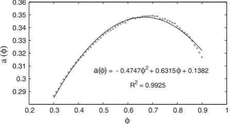
wherea(φ) can be approximated by a parabolic function ofφas shown in Fig.7. From the values ofa(φ)in Fig.7, the error in the estimation of the interface location is found to be of the order of magnitude of the square root of the permeability, which is commonly used as a characteristic length scale of the porous medium (e.g.,Kaviany 1995).
0 0.05 0.1 0.15
0 0.005 0.01 0.015 0.02 0.025 0.03 0.035 0.04 0.045 0.05
k (cm)
ξ(cm)0
0.3 0.4 0.5 0.6 0.7 0.9 φ
Fig. 6 The apparent interface location as a function of the square root of the permeability as calculated for a range of porosities
Fig. 7 The value ofa(φ)(Eq.18) as a function of porosityφ
0.2 0.3 0.4 0.5 0.6 0.7 0.8 0.9 1
0.29 0.3 0.31 0.32 0.33 0.34 0.35 0.36
φ
a (
φ)
a(φ) = - 0.4747 φ2 + 0.6315 φ + 0.1382
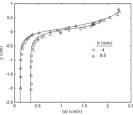
[image:11.439.106.333.275.454.2] [image:11.439.170.394.493.613.2]Fig. 8 A comparison between the macroscopic velocity profiles obtained by the apparent interface approach (solid lines) and PIV velocity data measured
byRosenzweig and Shavit(2007)
(symbols)
0 0.5 1 1.5 2 2.5
-2.5 -2 -1.5 -1 -0.5 0 0.5 1
<
u>
(cm/s)y (cm)
4 8.5
h (mm)
5.2 Comparisons with PIV Measurements
To verify the apparent interface approach, a comparison was made between its solutions and PIV (Particle Image Velocimetry) measurements obtained byRosenzweig and Shavit(2007) and byAgelinchaab et al.(2006). A comparison between the apparent interface approach and the results of these two studies is appropriate since the geometry used exhibits a sudden change in the porosity while moving across the interface, exactly as in the Taylor brush configuration.
Rosenzweig and Shavit(2007) modeled a porous domain by using a three dimensional Sierpinski carpet configuration which was made of transparent square columns. Figure8 shows a comparison between the superficial average velocity profile obtained by the apparent interface approach and the results of the PIV experiments for two different water depths, 4 and 8.5 mm (Fig.7inRosenzweig and Shavit 2007). The solution was generated using the Sierpinski carpet porosity and permeability, the fluid viscosity and density, and the pressure gradient as reported byRosenzweig and Shavit(2007) and listed in Table1. Best fit was obtained by matching the maximum velocities at the top free boundary. For the data set of
h=8.5 mm, the measured velocity was taken as the average of the two upper values near the
boundary, since a smaller value was measured at the top. As shown in Fig.8, a good agreement was found between the apparent interface solution and the measured results, indicating that this approach may serve as a good tool for predicting the velocity profile using only one measured value—the top boundary velocity.
[image:12.439.171.391.54.243.2]Table 1 Flow parameters
φ k µ h dPf/dx Umax
( – ) (cm2) (g cm−1s−1) (cm) (g cm−2s−2) (cm s−1)
This work 0.3–0.9 0.0005–0.2 0.01 1 or 2 −0.01 –
Rosenzweig and Shavit(2007) 0.79 0.0237 1.0584 0.4 −15.5 1.8532
0.79 0.0237 1.0584 0.85 −5.5 2.24
Agelinchaab et al.(2006) 0.95 0.102 0.29135 1.098 −0.214 0.17
0.78 0.00626 0.29135 1.098 −0.5 0.29 0.51 0.00392 0.29135 1.098 −0.3 0.17
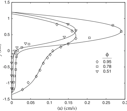
Fig. 9 A comparison between the macroscopic velocity profiles obtained by the apparent interface approach (solid lines) and PIV velocity data measured
byAgelinchaab et al.(2006)
(symbols)
0 0.05 0.1 0.15 0.2 0.25 0.3
-1.5 -1 -0.5 0 0.5 1 1.5
<
u>
(cm/s)y (cm)
0.95 0.78 0.51 φ
the valuesRosenzweig and Shavit(2007) report when comparing their results with those of Agelinchaab et al.(2006) (Fig.8inRosenzweig and Shavit 2007). Velocity profiles of the apparent interface approach were shifted upward by 0.5 and 1 mm to account for possible measurement errors in the PIV results reported byAgelinchaab et al.(2006). Similar to the first comparison, the results in Fig.9show that the apparent interface approach gives a good estimation of the velocity profile.
6 Conclusions
[image:13.439.174.391.189.378.2]An alternative approach is suggested, using an apparent interface for which both superficial velocity and intrinsic shear stress are continuous (i.e., β=0). The new approach shows advantages over previous approaches. First, the knowledge of the interface location is not needed. Furthermore, it can be easily applied knowing only the maximum velocity or the flow rate, which can be usually measured without much effort. The apparent interface approach is verified against PIV results from other works with much success, predicting the velocity profile for three-dimensional geometries that are more complex than the geometries of the current numerical and analytical investigation.
The apparent interface approach was developed and tested here for geometries with a sudden transition of the porosity between the porous domain and the free fluid. The apparent interface approach can also be applied for geometries with a gradual porosity transition; however, further research is needed to properly model the change in macroscopic parameters (such as the permeability) along the transition region.
Appendix A—Analytical Derivation of the Jump Condition Sensitivity to the Interface Location
Figure3a demonstrates that whenξ is small the calculated maximum velocity is a linear function ofξ. Equation17shows that the slope of this linear behavior is independent of the porous medium parameters, i.e.,φandk. In this appendix, we provide the justification for this result. We begin with Eq.16which was derived by substitution of theξinto the analytical solution of the macroscopic equations, Eqs.12–15(Sect. 4.2). It shows that the maximum velocity is a parabolic function of the parameterξ. As demonstrated in Fig.3a, it is clear that the parabolic term of Eq.16can be neglected for smallξ. In fact, whenξ is zero (i.e., nominal interface position) andβis given, Eq.16provides and expression for the averaged microscopic solution (Umax),
u|ξy==0h =Umax= −
1 2µ
∂pf
∂x
h2+2k(λ+1) (A1)
As defined in Sect. 4.1, we defineUmaxas the ‘true’ maximum velocity generated by
averaging the microscopic velocity at y = h. By using Eqs. A1 and16, the calculated maximum velocity can be approximated now as
u|y=h ≈ 1
µ ∂pf
∂x
h+
√
k
1/√φ−β
ξ+Umax (A2)
To simplify Eq.A2we use an order of magnitude analysis. For the porous media in this work,φ=O(1),β=O(1)andk<O(0.1 cm). Therefore,
√
k
1/√φ−β =O( √
k) (A3)
When the free water depth (h) is an order of magnitude higher than√k, the expression in Eq. A3 can be neglected from Eq.A2 and the deviation in the calculated maximum velocity (u|y=h) from its ‘true’ value (Umax) is expressed as written in Eq.17. In fact,
which means that the sensitivity of the model to the interface location is the same for any porous medium under these assumptions.
Appendix B—Analytical Solution of the Macroscopic Equations with Bounded Boundaries
The problem solved here is flow above porous medium bounded on top and bottom by an impermeable wall. The solution for this case is needed for a comparison with the measure-ments ofAgelinchaab et al.(2006). The governing equations of the problem are the same as those investigated in this work. The flow in the fluid domain is described by the Stokes equation (Eq.7), while the porous domain flow is governed by the Darcy–Brinkman equation (Eq.2) withµeff=µ/φ. The boundary conditions are zero velocity aty=handy= −D.
Continuity at the interface is applied on both superficial velocity and effective stress (Eq.3 withβ=0).
The velocity profile for the free fluid domain (y≥0) is
u(y)= 1
2µ dpf
dx y 2−
1 2µ
dpf
dx h+
u|y=0 h
y+ u|y=0, 0≤y≤h (B1)
The velocity profile in the porous domain (y≤0) is
u(y)= − k
µ dpf
dx +C1e
−y√φ/k+C 2ey
√
φ/k, −∞ ≤y≤0 (B2)
With the constants:
C1= 1 µddpxf ·
e−D√φ/k·
k−h22
+k·
h
√
φk +1
eD√φ/k·√h φk +1
+e−D√φ/k·√h φk−1
(B3)
C2= 1 µddpxf ·
k−h22
+C1·
h
√
φk−1
h
√
φk+1
(B4)
u|y=0 = −k
µ dpf
dx +C1+C2 (B5)
References
Agelinchaab, M., Tachie, M. F., Ruth, D. W.: Velocity measurement of flow through a model three-dimensional porous medium. Phys. Fluids18(2006) doi:10.1063/1.2164847
Beavers, G.S., Joseph, D.D.: Boundary conditions at a naturally permeable wall. J. Fluid Mech.30, 197– 207 (1967)
Breugem, W.P., Boersma, B.J.: Direct numerical simulations of turbulent flow over a permeable wall using a direct and a continuum approach. Phys. Fluids17. doi:025103(2005)
Breugem, W., Boersma, B.J., Uittenbogaard, R.E.: The laminar boundary layer over a permeable wall. Trans. Porous Media59, 267–300 (2005)
Chandesris, M., Jamet, D.: Boundary conditions at a planar fluid-porous interface for a Poiseuille flow. Int. J. Heat Mass Transfer49, 2137–2150 (2006)
du Plessis, J.P., Masliyah, J.H.: Mathematical modeling of flow through consolidated isotropic porous media. Trans. Porous Media3, 145–161 (1988)
Finnigan, J.: Turbulence in plant canopies. Annu. Rev. Fluid Mech.32, 519–571 (2000)
Goyeau, B., Lhuillier, D., Gobin, D., Velarde, M.G.: Momentum transport at a fluid-porous interface. Int. J. Heat Mass Transfer46, 4071–4081 (2003)
Kaviany, M.: Principles of Heat Transfer in Porous Media, 2nd edn. Springer, New York (1995)
Kuznetsov, A.V., Xiong, M.: Development of an engineering approach to computations of turbulent flows in composite porous/fluid domains. Int. J. Therm. Sci.42, 913–919 (2003)
Larson, R.E., Higdon, J.J.L.: Microscopic flow near the surface of two-dimensional porous-media. 1. Axial-flow. J. Fluid Mech.166, 449–472 (1986)
Larson, R.E., Higdon, J.J.L.: Microscopic flow near the surface of two-dimensional porous-media. 2. Trans-verse flow. J. Fluid Mech.178, 119–136 (1987)
Lowe, R.J., Shavit, U., Falter J.L., Koseff, J.R., Monismith, S.G.: Modeling flow in coral communities with and without waves: a synthesis of porous media and canopy flow approaches. Limnol Oceanogr.53(6), 2668–2680 (2008)
Lundgren, T.S.: Slow flow through stationary random beds and suspensions of spheres. J. Fluid Mech.51, 273– 299 (1972)
Neale, G., Nader, W.: Practical significance of Brinkmans extension of darcys law—coupled parallel flows within a channel and a bounding porous-medium. Can. J. Chem. Eng.52, 475–478 (1974)
Nield, D.A.: The limitations of the Brinkman-Forchheimer equation inmodeling flow in a saturated porous-medium and at an interface. Int. J. Heat Fluid Flow12, 269–272 (1991)
Ochoa-Tapia, J.A., Whitaker, S.: Momentum-transfer at the boundary between a porous-medium and a homo-geneous fluid. 1. Theoretical development. Int. J. Heat Mass Transfer38, 2635–2646 (1995a) Ochoa-Tapia, J.A., Whitaker, S.: Momentum-transfer at the boundary between a porous-medium and a
homo-geneous fluid. 2. Comparison with experiment. Int. J. Heat Mass Transfer38, 2647–2655 (1995b) Richardson, S.: A model for boundary condition of a porous material. Part 2. J Fluid Mech.49, 327–336 (1971) Rosenzweig, R., Shavit, U.: The laminar flow field at the interface of a Sierpinski carpet configuration. Water
Resour. Res.43. doi:10.1029/2006WR005801(2007)
Saffman, P.G.: On the boundary condition at surface of a porous medium. Stud. Appl. Math.50, 93–101 (1971) Sahraoui, M., Kaviany, M.: Slip and no-slip velocity boundary-conditions at interface of porous, plain
media. Int. J. Heat Mass Transfer.35, 927–943 (1992)
Saleh, S., Thovert, J.F., Adler, P.M.: Flow along porous-media by partial image velocimetry. AIChE J.39, 1765– 1776 (1993)
Shavit, U., Bar-Yosef, G., Rosenzweig, R., Assouline, S.: Modified Brinkman equation for a free flow problem at the interface of porous surfaces: the Cantor–Taylor brush configuration case. Water Resour. Res.38(12), 1320–1334 (2002)
Silva, R.A., de Lemos, M.J.S.: Numerical analysis of the stress jump interface condition for laminar flow over a porous layer. Numer. Heat Tr. A-Appl43, 603–617 (2003a)
Silva, R.A., de Lemos, M.J.S.: Turbulent flow in a channel occupied by a porous layer considering the stress jump at the interface. Int. J. Heat Mass Transfer46, 5113–5121 (2003b)
Taylor, G.I.: A model for boundary condition of a porous material. Part 1. J. Fluid Mech.49, 319–326 (1971) Valdes-Parada, F.J., Goyeau, B., Ochoa-Tapia, J.A.: Jump momentum boundary condition at a fluid-porous