Uncertainty and sensitivity in optode-based shelf-sea net community production estimates

www.biogeosciences.net/13/943/2016/ doi:10.5194/bg-13-943-2016

© Author(s) 2016. CC Attribution 3.0 License.

Uncertainty and sensitivity in optode-based shelf-sea net

community production estimates

Tom Hull1,2, Naomi Greenwood1,2, Jan Kaiser2, and Martin Johnson1,2 1_{Centre for Environment, Fisheries and Aquaculture Science, Lowestoft, UK}

2_{Centre for Ocean and Atmospheric Sciences, School of Environmental Sciences, University of East Anglia, Norwich, UK} Correspondence to: Tom Hull ([email protected])

Received: 27 August 2015 – Published in Biogeosciences Discuss.: 21 September 2015 Revised: 14 January 2016 – Accepted: 7 February 2016 – Published: 19 February 2016

Abstract. Coastal seas represent one of the most valuable and vulnerable habitats on Earth. Understanding biologi-cal productivity in these dynamic regions is vital to under-standing how they may influence and be affected by climate change. A key metric to this end is net community produc-tion (NCP), the net effect of autotrophy and heterotrophy; however accurate estimation of NCP has proved to be a dif-ficult task. Presented here is a thorough exploration and sen-sitivity analysis of an oxygen mass-balance-based NCP es-timation technique applied to the Warp Anchorage monitor-ing station, which is a permanently well-mixed shallow area within the River Thames plume. We have developed an open-source software package for calculating NCP estimates and air–sea gas flux. Our study site is identified as a region of net heterotrophy with strong seasonal variability. The annual cu-mulative net community oxygen production is calculated as (−5±2.5) mol m−2a−1. Short-term daily variability in oxy-gen is demonstrated to make accurate individual daily esti-mates challenging. The effects of bubble-induced supersatu-ration is shown to have a large influence on cumulative an-nual estimates and is the source of much uncertainty.

1 Introduction

Marine areas play a fundamental role in the cycling of carbon (Keeling and Shertz, 1992). Photo-autotrophic marine organ-isms fix CO2into organic matter. This organic matter is ex-ported from surface waters by the biological and solubility carbon pumps (Stanley et al., 2010).

Understanding the mechanisms driving these processes is vital for predicting how marine waters will respond to and

influence climate change (Guo et al., 2012; Palevsky et al., 2013). Coastal regions in particular have high value to soci-ety but are also vulnerable to anthropogenic activities (Jick-ells, 1998). These regions, which are typically more dynamic than the open ocean and have extensive natural variability, re-main a challenge for numerical models (Polton et al., 2013). The accurate detection and prediction of long-term trends, and any response in coastal ecosystems to changing environ-mental conditions, require the accurate capture of this vari-ability (Blauw et al., 2012). Effective ecosystem-based man-agement of these vital regions requires adequate monitoring, which drives the high demand for good-quality, cost-effective observations of environmental status indicators (Platt and Sathyendranath, 2008).

The balance between dissolved inorganic carbon (DIC) fixation (i.e. autotrophy) and production of DIC through het-erotrophy over a specified period is known as net community production (NCP; Williams, 1993). Net autotrophic systems occur when gross primary production is greater than respira-tion, and net heterotrophic systems occur when respiration is greater than primary production (Ostle et al., 2014).

ob-serving changes in CO2difficult. By comparison O2can be measured accurately and at high resolution over long periods with relative ease (Wikner et al., 2013).

Estimating net community production rates in the ocean is notoriously difficult (Williams et al., 2013; Duarte et al., 2013). This is in part because the net state is finely bal-anced between large opposing fluxes and measurements have large uncertainties (Ducklow and Doney, 2013). Approaches have broadly fallen into three categories: in vitro incu-bation experiments, ocean colour remote-sensing products, and in situ geochemical mass-balance methods. Mouriño-Carballido and Anderson (2009) noted that with in vitro in-cubation experiments the captured biota may not exhibit the same behaviour as they would in situ. Furthermore bottle samples may be spatially disparate from the source of pro-duction. For instance, where deep chlorophyll maxima form, the organisms of interest may not be captured unless specifi-cally targeted (Weston, 2005).

Karl et al. (2003) suggested that short, intensive bursts of photosynthesis driven by short-duration changes in light climate are regularly missed with traditional sampling tech-niques. Kaiser et al. (2005) also concluded that bottle incuba-tions are not suitable to correctly represent the net metabolic balance over larger temporal and spatial scales.

The remote sensing of NCP via ocean colour is in its in-fancy and requires calibration against reliable in situ mea-surements (Tilstone et al., 2015; Reuer et al., 2007). These methods are further hampered by insufficient spatial and tem-poral resolution or obscuring cloud cover (Thomas et al., 2002). Satellites only observe surface waters; they are thus unable to observe the deep chlorophyll maximum, which can contribute up to 60 % of the primary production (Fernand et al., 2013).

Given that production is episodic rather than continuous (Emerson et al., 2008) and the sites of increased production are patchy in nature (Alkire et al., 2012), high temporal res-olution in situ sampling is needed (Blauw et al., 2012)

Oxygen mass-balance techniques utilise measured changes in oxygen saturation and attempt to quantify the biological contribution to those changes in saturation. The approach to teasing apart the physical and biological drivers to these saturation changes can be subdivided into two groups: those which use a biologically inert analogue to oxy-gen, typically argon (Kaiser et al., 2005), and those which utilise gas solubility/transfer parametrisations to estimate air–sea exchange. The dual measurement of oxygen and an inert analogue tracer allows determination of solubility changes with fewer uncertainties than using gas solubility parametrisations; however the equipment required for this is not yet in widespread use.

The gas transfer parameterisation approach can be applied to historic data sets; given that the concentration of dissolved oxygen is the most widely measured property of seawater after temperature and salinity (McNeil and D’Asaro, 2014),

oxygen-based methods offer many opportunities to reveal new insights into data collected for other purposes.

To date, the majority of oxygen-based NCP estimates have focused on oceanic waters (Alkire et al., 2012). Emerson (2014) noted that coastal NCP values can be 3 times greater than open-ocean values; however, there are too few measure-ments to be confident in geographical variability. Palevsky et al. (2013) also found during their Gulf of Alaska O2/Ar survey that the transitional coastal zone contributed 58 % of the total NCP whilst representing only 20 % of the total area surveyed. The nature of the metabolic balance is partic-ularly important in river-dominated margins, where high car-bon and nutrient inputs stimulate primary production and mi-crobial respiration with large seasonal variations (Guo et al., 2012).

The Cefas (Centre for Environment, Fisheries and Aqua-culture Science) SmartBuoy network consists of autonomous data collection moorings placed at key locations in the UK shelf seas (Mills et al., 2005; Greenwood et al., 2010). The long-term, high-temporal-resolution multi-parameter data sets produced by the programme provide unique opportu-nities for observing biogeochemical processes in temperate coastal and shelf seas (Neukermans et al., 2012; Blauw et al., 2012; Foden et al., 2010).

In this paper we present new estimates of NCP from a long-term SmartBuoy mooring situated in the southern North Sea. We explore the uncertainty in these estimates and their sensitivity to uncertain input parameters. Lastly we make our algorithms available as open-source tools for readers to per-form their own NCP calculations.

2 Methods 2.1 Study site

The SmartBuoy sensor package consists of a Cefas ESM2 data logger coupled with Falmouth Scientific OEM conduc-tivity and temperature sensors (Falmouth Scientific, USA), an Aanderaa 3835 series optode (Aanderaa Data Instru-ments, Norway), a chlorophyll fluorometer (Seapoint Inc., USA), and a quantum photosynthetically active radiation me-ter (PAR; LiCor Inc., USA). The ESM2 includes a three-axis roll and pitch sensor with a internal pressure sensor (PDR1828 – Druck Inc). The data logger was configured to sample for a 10 min burst every half hour. Salinity, temper-ature, chlorophyll, and PAR are sampled at 1 Hz during the measurement period; oxygen is sampled at 0.2 Hz.

mix-Warp SmartBuoy

Sheerness tide gauge

51.0 51.5 52.0 52.5

−0.5 0.0 0.5 1.0 1.5 2.0

Depth (m) >200 100−200 50−100 25−50 <25

Figure 1. Map of Warp Anchorage study site.

Table 1. Study site characteristics for wWinter (November–

February) and sSummer (June–September), based on multi-year seasonal means.

Warp Anchorage

Position (WGS84) 51.31◦N, 1.02◦E

Monitoring Period 2001–present

Mean water depth (m) 15

Tidal range (m) 4.3

Tidal period semidiurnal

Salinity (PSS-78) 33.8w–34.3s

Turbidity (FTU)* 29w–10s

Temperature (◦C) 7.6w–17.5s

∗_{FTU: formazin turbidity units, ISO 7027.}

ing, together with the shallow water depth, has important im-plications to the application of oxygen-based NCP methods, which will be discussed later. The main characteristics of the study site are summarised in Table 1.

2.2 Data processing

SmartBuoy data undergo rigorous automated and manual quality assurance processes. Automated processes apply a quality flag to data which fall outside realistic value bounds. Manual processes assess the instrument performance and ap-ply flags where the data quality is compromised, e.g. due to biofouling or sensor damage. The CT sensor salinity data are corrected using in situ bottle samples analysed using a Guildline Portsal 8410A (Guildline, Canada) standardised with IAPSO standard seawater.

5 10 15

0 5 10 15

ECMWF

Ship anemometer

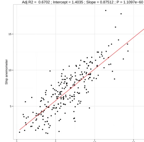
Adj R2 = 0.6702 ; Intercept = 1.4035 ; Slope = 0.87512 ; P = 1.1097e−60

Figure 2. Validation of ECMWF MACC reanalysis 10 m wind speed vs. height-corrected shipborne anemometer wind speed.

Water depth was calculated using a global tidal model forced with European shelf area constituents (TPX08-atlas). Tidal waves have been shown to arrive almost simultane-ously at both the Sheerness and the Warp SmartBuoy site (Blauw et al., 2012); thus model output was validated against the nearby Sheerness tide gauge (UK National Tide Gauge Network) and demonstrated good agreement visually. Wind-speed and sea level air pressure were taken from ECMWF MACC (Monitoring Atmospheric Composition and Climate) reanalysis with a 0.125◦ _{grid. ECMWF data were found to}

compare well with in situ shipborne anemometers used dur-ing moordur-ing servicdur-ing (see Fig. 2). Details of the ECMWF and tidal model validations and their bearing on the sensitiv-ity analysis are discussed later.

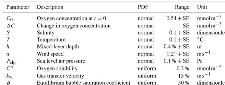
Table 2. Parameters and their uncertainty distributions used for LHS/PRCC and eFAST at the Warp site.

Parameter Description PDF Range Unit

C0 Oxygen concentration att=0 normal 0.54+SE mmol m−3

1C Change in oxygen concentration normal SE mmol m−3

S Salinity normal 0.1+SE dimensionless

T Temperature normal 0.1+SE ◦C

h Mixed-layer depth normal 0.4 %+SE m

u Wind speed normal 1.2∗+SE m s−1

Pslp Sea level air pressure normal 0.1 %+SE Pa

C∗ Oxygen solubility uniform 0.3 % mmol m−3

kw Gas transfer velocity uniform 15 % m s−1

B Equilibrium bubble saturation coefficient uniform 50 % dimensionless

SE: the standard error of the mean.

2.3 Optodes

Aanderaa Instruments model 3830 and 3835 optodes (Aan-deraa, Norway) have been fitted to the Cefas SmartBuoys since 2005. Optodes drift due to foil photobleaching in a predictable way (Tengberg et al., 2006), which is well de-scribed by a decaying exponential with a decay constant of approximately 2 years (McNeil and D’Asaro, 2014). All op-todes used were fitted with the opaque black silicon pro-tective coating. Thus drift is significantly reduced after a burning-in period, and the temperature correction is unaf-fected (D’Asaro and McNeil, 2013). Sensor drift was cor-rected with an offset calculated from frequent discrete sam-ples measured with volumetric Winkler titrations (Hansen, 1999). Titrations were performed using an automatic pho-tometric end-point detection system (Metrohm Dosimat 665 Autotitrator); the thiosulfate is intermittently standardised with a standard potassium iodate solution (Wiliams and Jenk-inson, 1982). The classical Winkler method if executed with care by a skilled operator offers very low uncertainty (Helm et al., 2009), typically better than 0.2 % (Emerson and Stump, 2010; Ostle et al., 2014). It is however a demanding task that is affected by numerous uncertainty sources, such as contam-ination of the sample and reagents by atmospheric oxygen and iodine volatilisation. Photometric end-point detection is further affected in highly turbid waters, which can limit the number of successful samples.

2.4 Model implementation

NCP is calculated here using a modified version of the zero-dimensional oxygen mass-balance (box) model of Emerson (1987) and Emerson et al. (2008). This describes the oxy-gen mass balance in the mixed layer, assuming no vertical or horizontal advection and no turbulent diffusion across any mixed-layer boundary.

Given that the Warp site is permanently mixed, there is in effect direct connection between the atmosphere and the benthos. It is thus an important distinction from prior studies

that our community productivity estimate considers both the pelagic and benthic processes as one system. This method assumes that other oxygen-consuming processes in the water column such as nitrification, methanotrophy, and photoox-idation are negligible relative to respiration (Reuer et al., 2007). In our discussion we explore the implications for a site, such as the Warp site, where all of these assumptions may not hold.

The model (Eq. 1) is used to predict the concentration of oxygen at a subsequent point in time given measured phys-ical parameters. Any deviation from the predicted value is assumed to be from biological activity, with a positive value corresponding to net production. This method of NCP es-timation makes no distinction between matter which is im-ported then locally respired and that which is fixed locally. All of these terms introduced below and their estimated un-certainties are summarised in Table 2.

hdC

dt =E+G+J, (1)

wherehis the mixed-layer depth,Cis the oxygen concentra-tion in the mixed layer,Eis entrainment of oxygen through changes in the mixed-layer depth (Eq. 2),Gis the gas ex-change through diffusive and bubble processes (Eq. 3), and

Jis the net community production.

E=dh

dt(Cb−C), (2)

whereCbis the oxygen concentration below the mixed layer.

G=kw

(1+B)Pslp Patm

C∗−C

, (3)

using the Benson and Krause (1984) data,B is supersatura-tion caused by bubble processes (Eq. 5), andPslpis sea level pressure,Patmis standard atmospheric pressure (101 325 Pa).

kw=0.251U2

_Sc

O2 660

−0.5

, (4)

whereU is the wind speed at 10 m andScO2 is the dimen-sionless Schmidt number for oxygen. The typically quoted Schmidt number for CO2 at 20◦C in salt water (S=35) is 660. Note the result of Eq. (4) is converted from cm h−1 to m s−1for use in Eq. (3).

The square root of the squared mean was used for wind speed to fit with the quadratickwparametrisation used. Wan-ninkhof et al. (2009) argue that comprehensive surface forc-ing models provide little to no improvement over simple wind speed algorithms, and although simple parametrisations cannot capture all the processes that control gas transfer, they appear to capture most.

The injection of bubbles into the mixed layer through wave action can supersaturate the surface waters even if net gas exchange is zero (Liang et al., 2013). Here we utilise a mod-ern kw parametrisation with an explicit bubble equilibrium fractional supersaturation parametrisationB, which enables the influence of the two elements on the NCP estimate to be quantified independently. ForB the bubble supersaturation parametrisation of Woolf and Thorpe (1991) is used:

B=0.01·

_U

Ui 2

, (5)

whereUi is the wind speed at which the equilibrium super-saturation is 1 %. For oxygen Woolf and Thorpe (1991) re-port this value to be 9 m s−1.

Liang et al. (2013) argue that bubble supersaturation effects at a given temperature differ significantly among parametrisations, and their comparison between Stanley et al. (2009), Woolf and Thorpe (1991), and their own parametrisa-tion demonstrates differences in the order of 50 % for argon. The Woolf and Thorpe (1991) parametrisation does not ac-count for any temperature or solubility dependence and is de-rived from calculated bubbled fields; implementation is how-ever straightforward and the large relative uncertainties in the bubble term will be accounted for in the sensitivity analysis outlined below.

We solve Eq. (1) for NCP (J) using the analytical solu-tion shown in Eq. (6), providing mean values for each vari-able except oxygen concentration and assuming a constant rate of NCP over the time step, which for this study cor-responds to 25 h. The numerical scheme used in this paper was implemented using R, the opsource language and en-vironment for statistical computing (R Foundation for Sta-tistical Computing, www.r-project.org). The analytical solu-tion along with kw and B parametrisations are included in the “airsea” package (Hull and Johnson, 2015). The scheme

was validated in silico using numerical estimation; air–sea fluxes were simulated every half second forced with a known value of NCP; the resultant change in oxygen concentration was provided to our model; and the calculated value of NCP compared to the known forced value. This was repeated over a range of input scenarios.

J=rh

_C

1−C0 1−e−rt +C0

−F h, (6)

whereC0is the oxygen concentration at the initial time step (t=0), andC1is the concentration att.

r=kw

h +

1

h

dh

dt (7)

F =kw

h C

∗

(1+B)Pslp Patm

+1

h

dh

dtCb (8)

It should be noted that for this study the entrainment (d_dh_t) term is neglected as the Warp site is a perpetually fully mixed site; as such the entrainment term of Eqs. (7) and (8) are set to 0.

2.5 Sensitivity analysis methods

Accurately assessing the sensitivity of a model output to un-certain input variables has many uses. Primarily it is to de-termine the precision of the model output and the sources of output uncertainty, knowledge of which informs future re-search in targeting the main sources of uncertainty if robust-ness is to be increased (Saltelli et al., 2000).

Local sensitivity analysis methods, such as the so-called one-at-a-time techniques, are limited to providing informa-tion only in a very specific locainforma-tion of the parameter space. These methods rely on the selection of an applicable baseline and varying a single input parameter, which ignores the ef-fects of covariant parameter uncertainty (Saltelli et al., 2000). Global methods such as Latin hypercube sampling with partial rank correlation coefficients (LHS/PRCCs) and the extended Fourier amplitude sensitivity test (eFAST) are ca-pable of assessing multiple locations across the entire param-eter space; thus covariant paramparam-eter uncertainty is captured.

but one of the variables. A simple one-at-a-time analysis re-veals that the variables do indeed demonstrate the monotonic relationships required for effective PRCCs. eFAST provides first- and total-order Sobol indices which indicate the vari-ance of the conditional expectation of the output for a given variable (Saltelli et al., 2000).

LHS is performed by assigning a error probability density function (PDF) to each of the parameters. Each PDF is split intonequiprobable divisions, and each area randomly sam-pled once without replacement. This table of input variables is then used to calculate NCP, with a new hypercube being generated for each time step. A column-wise, pair-wise al-gorithm is then used to generate an optimally designed hy-percube, where the mean distance between each point and all other points in the hypercube is maximised (Stocki, 2005). We utilise the “improved” LHS implementation within the “lhs” R package (Carnell, 2012) together with the PRCC rou-tine from “epiR” (Nunes et al., 2014). The eFAST scheme is provided by the “sensitivity” package (Pujol et al., 2014).

While there is no a priori exact rule for determining sen-sible sample size for these methods, minimum values are known to ben=k+1 for LHS/PRCC andn=65 for eFAST (Saltelli et al., 2000), wherek is the number of parameters. Here we took the usual approach of systematically increas-ing sample size and checkincreas-ing if the sensitivity index is con-sistent at least for the main effects, thus demonstrating there is no advantage to increasing sample size as the conclusions remain the same.

LHS/PRCC and eFAST analyses were run 500 times for each 25 h step of the time series, and the results were aggre-gated. For cumulative calculationskw,B, andC∗and the bias element of each measurement parameter were applied glob-ally for the entire time series; that is to say a single hyper-cube (n=500) is used to set the bias and scaling factors for multiple runs over the entire time series, while the stochastic uncertainties are applied at each time step independently. 2.6 Uncertainty distributions

Critical to the value of any sensitivity or uncertainty analysis is the selection of adequate probability distribution functions for each input parameter (Marino et al., 2008). Table 2 sum-marises the probability distribution functions used for each of the NCP model input parameters.

The two oxygen terms (C0,1C) were determined through replicate anchor station Winkler samples taken close to the mooring during maintenance surveys, combined with an es-timate of Winkler method error and water bath tests of optode precision.C0represents the precision and accuracy of the ini-tial (t=0) oxygen concentration. We estimate this residual standard error in oxygen determination from the corrected optode, combined with the accuracy of the Winkler samples, to be within±0.52 mmol m−3. The error bounds for1C, un-like the other measured parameters, are derived solely from the standard error of the difference between the oxygen

con-centration at each time time step. This standard error rep-resents both the variability within each 25 h mean and the precision of the optode.

The calculation ofkw is conservatively assumed to be ac-curate to±15 % (Wanninkhof, 2014). The root-mean-square error (RMSE) from regressions between ECMWF and ship anemometer, shown in Fig. 2, is used to give an estimated wind speed error. For salinity we use the RMSE between the corrected CT, as detailed above, and the bottle samples (0.1). Water bath calibrations have confirmed the SmartBuoy temperature sensors to be accurate to within±0.1◦C. Gar-cía and Gordon (1992) provide an uncertainty estimate for the measurement of their oxygen solubility parameterisation of 0.3 %. We have selected a 50 % uniform uncertainty dis-tribution forB, the equilibrium bubble supersaturation term, based on the assessment of parametrisations by Liang et al. (2013).

At the Warp site, given the assertion that it is always fully mixed, the uncertainty inhis reduced to an estimate for the inaccuracies in the tidal model.

Regressions between the predicted height from the model and the Sheerness tide gauge results in a RMSE of approxi-mately 0.4 %. These estimates of parameter measurement un-certainty were combined, using the square root of the sum of squares, with the standard error of each mean observed value. The uniform bias was found to be relatively small compared to the observed standard errors, and thus the overall parame-ter error is considered to be normally distributed.

Uncertainty distributions forkw,B, andC∗were applied by multiplying the parameterised output by a scaling factor sampled from a uncertainty probability distribution. This ren-ders the uncertainty in the parametrisation independent of the input parameters; i.e.kwuncertainty is independent ofu un-certainty.

3 Results 3.1 NCP

0 5 10 15 20

0 50 100 150

0 5 10 15 20

Jan Feb Mar Apr May Jun

Jan Feb Mar Apr May Jun

Jan Feb Mar Apr May Jun

Chlo

rop

hyll

Fluo

roe

scence

(

Arb.

Unit

)

Oxygen satur

ation anomaly ( mmol

m

−

3 )

Wind Speed ( m

s

−

1 )

(a)

(b)

(c)

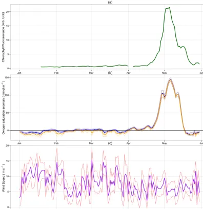
Figure 3. Spring 2008 Warp Anchorage time series. (a) Chlorophyll fluorometry. (b) Oxygen saturation anomaly (oxygen concentration mi-nus the solubility). Orange and blue lines represent oxygen saturation anomaly with and without bubble supersaturation effects respectively.

(c) ECMWF MACC reanalysis 10 m wind speed. For (b) and (c) thin lines represent 2σ confidence bounds.

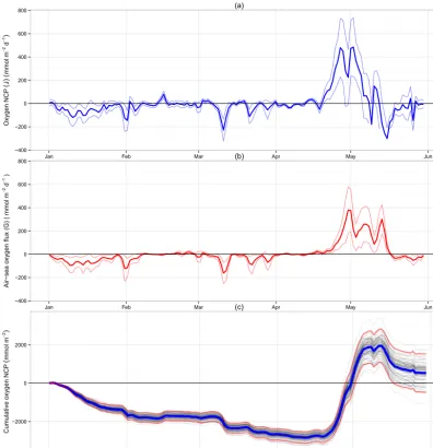
Figure 4a shows the calculated NCP for the spring 2008 study period at the Warp site.

All NCP values are given as oxygen equivalents unless otherwise stated. NCP is characterised by small, mostly neg-ative fluxes for the first 3 months. This is followed by a marked phytoplankton bloom (Fig. 3a) and resulting positive net community production lasting approximately 3 weeks. Large negative NCP is seen following the bloom, indicating enhanced community respiration. The observed NCP signal is in good agreement with chlorophyll fluorescence (Fig. 3a). The maximum rate of net community oxygen produc-tion was calculated as (485±129) mmol m−2d−1 with 2σ

confidence and precedes maximum observed chlorophyll by 3 days. The mean rate during the non-productive period (January–April) is estimated as (−30±9.5) mmol m−2_d−1_.

The maximum rate of O2influx from the atmosphere was (161±47) mmol m−2d−1, measured on 1 February 2008, which was concomitant with 14 m s−1winds (Fig. 3c) and a

−2.5 mmol m−3oxygen anomaly. The maximal rate of oxy-gen out-gassing was observed on 1 May 2008 of (380±102) mmol m−2d−1 after the initial peak of the phytoplankton bloom.

−400 −200 0 200 400 600 800

−400 −200 0 200 400 600 800

−2000 0 2000

Jan Feb Mar Apr May Jun

Jan Feb Mar Apr May Jun

Jan Feb Mar Apr May Jun

O

xyge

n

NCP

(

J

)

(

mmol

m

−

2d

−

1)

Air−sea o

xygen flux (G) ( mm

ol

m

−

2d

−

1 )

Cum

ulative

oxygen

NCP

(

mm

ol

m

−

2)

(a)

(b)

(c)

Figure 4. Spring 2008 Warp Anchorage time series. (a) Net community production (J); negative values correspond to net respiration.

(b) Oxygen air–sea gas exchange (G); negative values correspond to movement into the sea. For (a) and (b) thin lines represent 2σconfidence

bounds. (c) Cumulative net community production, mean value shown in blue, each run shown in grey, 2σ confidence bounds in red.

−4000 −2000 0

Oct 01 Oct 15 Nov 01 Nov 15 Dec 01 Dec 15 Jan 01

C

u

m

u

la

ti

v

e

o

x

y

g

e

n

N

C

P

(

m

m

o

l

m

−

2)

−100 0 100

−100 0 100

−100 0 100

2008

2009

2010

Jun Jul Aug Sep Oct Nov

O

x

y

g

e

n

N

C

P

(

m

m

o

l

m

−

2d

−

1)

Figure 6. Warp June–October NCP estimates from other years demonstrating no significant periods of net production.

We estimate the cumulative NCP for the missing 4-month period of 2010 (July–October) using the mean rate for this period across other years of the 10-year Warp data set, a sub-set of which is shown in Fig. 6. We calculate the mean value (−18.2±2.3) mmol m−2d−1, giving a cumulative estimate for this period of (−2.2±0.4) mol m−2. There are no sig-nificant net autotrophic periods observed between June and September in any other year.

We thus determine that the Warp site is net heterotrophic with an annual oxygen NCP of (−5±2.5) mol m−2a−1. However the validity of this assertion is discussed further later.

3.2 Sensitivity

Figure 7a shows total-order Sobol indices for the same pe-riod computed with eFAST. Here “total” is given to mean the factors’ main effects on the NCP estimate, combined with all the interacting terms involving that factor as per Saltelli et al. (2000). The Sobol indices are normalised to the total vari-ance, giving an indication of the fractional contribution to the variance for each factor. Note that, unlike first- order in-dices, the sum of the total indices can exceed one; in Figs. 7a and 8 we have normalised the total-order indices to one to aid visualisation.

The squared PRCC values from spring 2008 are shown in Fig. 7b. These values are ranked measures, normalised to one, of the degree of monotonicity of each variable on NCP (Sanchez and Blower, 1997). In plainer terms, these are a measure of the independent effect of each input parameter on NCP regardless of whether any input parameter variables correlate. Using squared values makes for easier

compari-son with the eFAST indices as the ranked coefficients can be both negative and positive. The relationship between each of the variables and NCP is monotonic for the parameter ranges generated for each time step and thus each PRCC calculation. However, in aggregate over the data set some of the variables can demonstrate a positive and negative (non-monotonic) re-lationship with NCP.

Both techniques indicate the determination of the change in oxygen concentration (1C) has the largest influence on overall uncertainty, with both the highest PRCC ranking and Sobol total-order indices. The eFAST analysis indicates that

1C typically accounts for 53 % of the overall uncertainty. Wind speed u is the second-largest contributor, typically comprising 26 % of the uncertainty budget. The bubble su-persaturation parametrisationB accounts for 9 %. The gas transfer velocity parametrisation (kw) and the initial oxygen concentration accuracy (C0) are shown to have similar con-tributions of 6 %. The García and Gordon (1992) oxygen sat-uration parametrisation contributes 4 %. Similar results from both sensitivity analyses indicate the model is well charac-terised by these methods.

The large confidence limits shown for u, kw, and B in Fig. 7 illustrate the large variability in PRCC ranking and Sobol indices over the period studied. This indicates how the relative importance of these factors varies greatly over the data set. The timings for this variability is illustrated in Fig. 8. Here we observe periods (early January and most of March) where1C uncertainty is of minimal importance and wind speed uncertainty dominates. The uncertainty in NCP dur-ing the onset of the bloom (mid-April to mid-May) is almost completely dictated by uncertainty in1C.

LHS/PRCC is not suitable for assessing the effects of mea-surement and parameterisation bias on the cumulative NCP estimate. Uncertainty in some of the parameters, principally

uandkw, do not demonstrate monotonic relationships with the output measure. That is to say uncertainty inucan lead to both increased or decreased cumulative NCP. Thus we present only eFAST indices for cumulative uncertainty in Fig. 9.Bis shown to have the largest contribution, account-ing for 40 % of the uncertainty in NCP alone, with a further 7 % from interactions primarily withu.

4 Discussion 4.1 NCP

eFAST PRCC

0.00 0.25 0.50 0.75 1.00

C0 dC u S T h Pslp kw B C* C0 dC u S T h Pslp kw B C*

Figure 7. Warp sensitivity analysis indices. (a) eFAST total-order Sobol indices (fractional uncertainty contributions). (b) PRCC squared indices (ranked uncertainty contributions). Box plot upper and lower hinges correspond to first and third quartiles; whiskers extend to 1.5× of the inter-quartile range; outliers are marked with dots. See Table 2 for variable definitions.

0.00 0.25 0.50 0.75 1.00

Jan Feb Mar Apr May Jun

T

otal order eF

AST inde

x

B C0 dC kw Other u

Figure 8. Warp eFAST total-order Sobol indices over time, indicating changing fractional contributions to uncertainty from each of the main parameters.

26 mmol m−2d−1 in April (Trimmer et al., 2000). Braeck-man et al. (2014) observed maximal mean rates of nitrifica-tion reaching 6 mmol m−2d−1and similar for mineralisation in muddy coastal North Sea sediment. This combined with sediment respiration equated to a sediment community oxy-gen consumption of 15 for February and 20 mmol m−2_d−1 for April. This indicates that a large fraction (perhaps 50 %) of the observed negative NCP at the Warp site could be due to sedimentary processes.

It is important to consider that chemoautotrophic pro-cesses, such as nitrification, contribute positively to the metabolic balance but negatively to the oxygen inventory. This is true not just for benthically coupled sites like Warp but for any system where these processes occur. These pro-cesses, while assumed small relative to respiration and pho-toautotrophy by (Reuer et al., 2007) in the Southern Ocean, are likely more important for shelf-sea systems.

There are two events – one at the start of February, another in the second week of March – where high winds appear to coincide with increased negative NCP (Fig. 4a). This could

be considered non-intuitive as one may expect increased ven-tilation to drive the system closer to equilibrium, but this is not the case as shown in Fig. 3b. There are several pos-sible explanations. The optode may be underestimating, or the estimation of saturation concentration incorrect, while in truth the system is supersaturated and is being driven closer to equilibrium during the windy events. We think this un-likely given our error bounds, calibration procedures, and the results from our sensitivity analysis, which indicate the bulk of the contribution to uncertainty is from theu term (Fig. 8). The windy periods could be driving resuspension events which could induce the apparent negative NCP. Lastly, this could be an artefact of the bubble supersaturation term overestimating at high wind speed. The orange line of Fig. 3b shows the effects of the bubble term, and uncertainty, relative to the uncorrected blue line.

0.00 0.25 0.50 0.75 1.00

B C C* h Kw Pslp S T u

Figure 9. Warp eFAST first-order (red) and total-order (Cyan) Sobol indices for cumulative NCP, indicating relative contributions from parameter bias uncertainty to cumulative NCP uncertainty.

0 50 100 150

31 32 33 34

O

x

y

g

e

n

anomaly

(

m

m

o

l

m

−

3

)

S

a

lin

ity

Apr 01 Apr 15 May 01 May 15 Jun 01

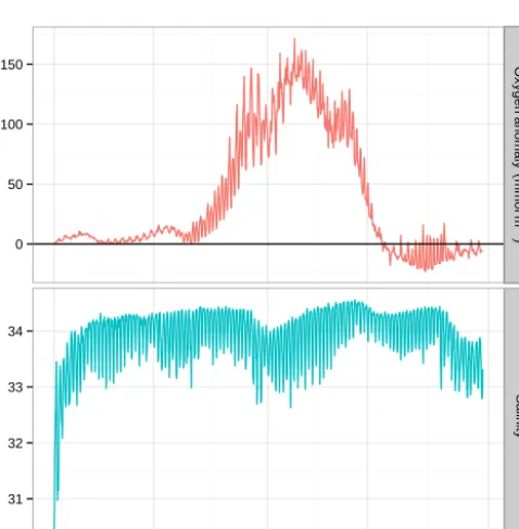
Figure 10. Raw (30 min) Warp SmartBuoy time series showing significant variability in oxygen anomaly (red) and salinity (blue) within each tidal cycle. Here the oxygen anomaly neglects the su-persaturating effects of bubbles.

the annual budget could indicate that annual estimates, while vital for carbon cycling studies, are a less useful indicator for

ecosystem health. A carefully resolved bloom period NCP may be more useful.

4.2 NCP as carbon equivalents

The commonly used “Redfield” stoichiometric ratio for O : C of 1.45 (Anderson and Sarmiento, 1994; Hedges et al., 2002) was applied to our positive oxygen NCP estimates for easier comparisons with other studies.

Literature values for NCP estimates from regions similar to the Warp site are scarce. Tijssen and Eijgenraam (1982) calculated net community oxygen production in the South-ern Bight of the North Sea using shipboard 4-hourly Winkler samples. They performed two surveys of 2–3 days in March and April 1980 with 24 h net community oxygen production estimates of 26 and 304 mmol m−2_d−1_{respectively.}

The rates of net production seen at the Warp site when expressed in units of carbon are of comparable magnitude to other estimates, with a maximal carbon NCP rate of (346±92) mmol m−2d−1. Guo et al. (2012) report similar magnitudes of peak NCP from other studies in large river plume regions.

Bozec et al. (2006) reported an annual carbon NCP esti-mate for the entire Thames plume region of 3 mol m−2a−1. Their study integrated their four seasonal survey tracks into ICES (International Council for the Exploration of the Sea) regions, of which the Thames plume is one. Our annual car-bon NCP estimate of (−3.6±1.8) mol m−2a−1represents a much smaller area, measured at considerably higher tempo-ral resolution, for a much longer duration.

4.3 Measurement and model uncertainty

Prior oxygen NCP studies have neglected to include the pro-duction of oxygen within the time step; that is to say they as-sume an instantaneous production of NCP at the end of their time step when the measured oxygen concentration and abi-otically predicted concentration are compared. This results in the underestimation of the magnitude of NCP. For exam-ple, oxygen produced at the start of the time step will out-gas quicker due to the increased air–sea concentration gradient, and when the degree of supersaturation is later measured at the end of the time step the true magnitude of the supersatu-ration will be masked.

The effect of neglecting the within-time-step NCP is negli-gible when conditions are near equilibrium saturation. How-ever, during the bloom, neglecting the within-time-step NCP would result in a 45 mmol m−2d−1(9 %) underestimation of peak oxygen NCP.

analy-sis of their O2/N2method where 54 % of the uncertainty was due to oxygen determination.

The mean and median value for1C standard error were 1.1 and 0.6 mmol m−3 respectively. Greater variability is seen during the bloom, with values up to 7.0 mmol m−3. During calibration in a thermostatic bath the optodes used typically demonstrated a precision of ±0.3mmol m−3. This is within the specification from the manufacturer of

±0.4 mmol m−3 and in agreement with the findings of Wikner et al. (2013). Thus it would appear that the largest source of uncertainty constrained here is the large degree of variability captured within the 25 h mean rather than the in-strument. The range of values observed within any 25 h pe-riod differed by up to 91.2 mmol m−3during the bloom. Dur-ing the non-productive period the observations within each 25 h period varied by on average 9.2 mmol m−3_{. This} vari-ability is shown with the small subsection of the raw oxygen time series presented in Fig. 10. The variability seen here represents both tidal movement of water past the buoy and diel cycling of production.

Thus we believe improvements in identifying homoge-neous water masses over the tidal cycle, rather than integrat-ing it entirely, is the best approach to reducintegrat-ing uncertainty with this scheme.

Shipboard transect studies (typically utilising O2/Ar methods in open-ocean environments) observe any disequi-librium oxygen in relation to the gas residence time; that is, they assume constant NCP in the period leading up to the measurement (Kaiser and Gist, 2006). It would thus appear that single shipboard transects will struggle to fully capture the tidally induced variability found in areas such as the Warp site.

For the investigation of cumulative uncertainty we con-sider only the bias in each parameter. The bubble supersatu-ration term (B), while small in regards to PRCC and eFAST values for an individual estimate (Fig. 7), has a large effect on the cumulative mass balance (Fig. 9). We calculate a pseudo-cumulative spring period NCP of (2.3±0.9) mol O2m−2 re-sulting from neglecting B: 4 times our true estimate. This relatively large effect is due to the biased nature of the su-persaturation term, which serves to only increase the oxygen concentration in the mixed layer.

Optodes tend to drift towards underestimating oxygen con-centrations (Wikner et al., 2013), which will typically re-sult in underestimates of NCP. We re-ran our analysis, sim-ulating a 1 mmol m−3_{per month negative linear drift, which} provides a pseudo-cumulative oxygen NCP estimate for the spring period of (−0.5±0.8) mmol m−2_{, which contrasts} with our corrected value of (0.5±1.0) mmol m−2. This re-inforces the requirement for well-calibrated, drift-corrected measurements.

Future studies are likely to benefit from newer optode de-signs than those used here. Together with the improved multi-point calibration equation (Stern–Volmer) of McNeil and D’Asaro (2014), these can offer greater accuracy and

pre-cision. The in-air calibration procedures outlined by Bushin-sky and Emerson (2013) can reportedly offer frequent in situ calibrations of±0.1 %. The in-air measurements could also be used to calculate the concentration gradient between the mixed-layer waters and the air, which eliminates the require-ment for aC∗parametrisation

Emerson et al. (2008) noted that at the Hawaii Ocean Time-Series site small daily fluctuations in the measured oxygen concentration caused large fluxes, but these were both positive and negative and had little impact on the cu-mulative NCP. Fluctuations around zero are seen at the Warp site. These do not tend to cancel out and combine to form a significant negative NCP flux. Emerson (2014) observed the standard deviation of the individual mean annual values is up to±50 %, which reflects both real inter-annual variability and measurement/model error. This study has produced NCP estimates for the spring period of up to almost 100 % due primarily to the large uncertainty centred around the bloom. Our winter period estimate demonstrates a degree of uncer-tainty similar to that of Emerson (2014) albeit with a net het-erotrophic system.

4.4 Advection and sampling uncertainty

Previous studies in open-ocean environments have ignored horizontal advection (Emerson et al., 2008; Nicholson et al., 2008). Air–sea gas exchange is typically considered to be sufficiently rapid that horizontal gradients are too small to drive a significant flux (Alkire et al., 2014). Semi-diurnal tidal systems such as at the Warp site demonstrate horizon-tal displacement of water masses with a periodicity of 12 h 25 min, with maxima in current speeds every 6 h 12 min, which drive significant horizontal variability (Blauw et al., 2012).

The box model presented here relies on the assumption that the instruments are measuring the same body of water twice; i.e. the comparison of two consecutive 25 h averages represents the same mass of water evolved over time.

If we assume that conditions along the path length are homogeneous on 25 h time scales, in effect the NCP esti-mates presented here can be thought of as integrating over a length scale proportional to the residual flow. Historic in situ acoustic Doppler current profiler data gathered over 3 months at the Warp site (see Appendix A) show a residual mean current flow estimated at 1.9–2.2 cm s−1, bearing 120◦. This combined with the average tidal excursion of 1.7 km d−1 equates to a observational window of approximately 3.5. km fort=25 h.

what extent patchiness within this timescale can influences our estimates is a further step to ensuring a robust NCP esti-mate.

Residual currents will also affect the NCP estimates by the addition and loss of water from outside of our observa-tional window. Alkire et al. (2014) calculated the advective flux during their glider study and observed daily mean flow of up to 2 cm s−2. This when combined with their measured horizontal gradient produced the mean removal of (18±10) mmol m−2d−1oxygen through horizontal advection.

We have attempted to estimate the oxygen concentration gradient from the tidally driven oxygen variability, that is, the difference between the oxygen concentration at low and high tide. We calculate this for our January period to be approxi-mately 2 mmol m−3, with low-tide concentration greater than that of high tide. From that we can estimate an advective flux of 51 mmol m−2_d−1_{using Eq. (9) (Emerson and Stump,} 2010).

AF =v

_dC

dx

h, (9)

wherevis the Ekman advection velocity.

This is not an insignificant flux relative to our calculated winter heterotrophy and would indicate that our site could actually be autotrophic with the heterotrophic processes oc-curring upstream. It is clear that consideration of advection is required to accurately estimate the annual metabolic state at this site.

4.5 Other sources of uncertainty

There are several other known contributors to NCP uncer-tainty which are outside the scope of this study. Kitidis et al. (2014) argue that all O2-based methods underestimate NCP due to photochemical processes, and they report that their modelled photochemical oxygen demand was shown to occa-sionally exceed respiration, with demand ranging between 3 and 16 mmol m−3d−1. Oxygen photolysis was found to cor-relate with chromophoric dissolved organic matter (CDOM) absorbance at 300 nm. While significant concentrations of CDOM can be found at the Warp site (Foden et al., 2008), the effects are likely mitigated by the typically high turbid-ity, the associated rapid light attenuation, and shallow (fre-quently < 6 m) photic depth.

Tijssen and Eijgenraam (1982) observed, in the northern end of the Southern Bight of the North Sea in April, ver-tical oxygen gradients of up to 0.15 mmol m−3. These can form throughout the day during the phytoplankton bloom. The gradient was reversed during the night, indicating the re-distribution of oxygen by vertical mixing over a 24 h period.

Takagaki and Komori (2007) found the maximum en-hancement to CO2gas transfer by rainfall is similar in mag-nitude to that of high wind speeds. This enhancement is thought mainly to be through increased turbulence and sur-face area at the air–water intersur-face, and as such it is likely to be most significant where heavy rain is coincident with light winds (Beale et al., 2013).

Frew (1997) found that surfactants may be responsible for coastal waters having significantly lower transfer velocities than oligotrophic areas. However Nightingale et al. (2000) found no measurable change inkwduring a 30-fold increase in chlorophyll during an algal bloom. We, like Wanninkhof et al. (2009), consider that practically surfactants are always in effect and are thus incorporated into empirically derived

kwparametrisations.

Similarly while sea spray may also enhance gas trans-fer, we believe this to also already be accounted for in the parametrisation. Further uncertainties relating to the parametrisation ofkware likely of little concern without first reducing other, more significant sources.

5 Conclusions

Our work identifies the Warp SmartBuoy site as an annu-ally net heterotrophic location with strong seasonal variabil-ity and autotrophy during the growth phase of the bloom. However, this assertion is brought into question due to signif-icant unconstrained uncertainties from horizontal advection, the determination of which is outside the scope of this study. We have demonstrated that the largest constrained source of uncertainty in our NCP estimates comes not from the se-lection of gas exchange parametrisation, or the quality of remote-sensed and modelled parameters, but from the mea-surement of the changing oxygen concentration. For cumu-lative annual estimates, the strongly biasing uncertainty of bubble-induced supersaturation is the dominant source of un-certainty.

Appendix A

0 5 10

0 5 10

EAST

NOR

TH

Dec 16 00:00 Dec 16 06:00 Dec 16 12:00 Dec 16 18:00 Dec 17 00:00

Height (m)

−1.0 −0.5 0.0 0.5 1.0 Velocity (m s−1)

Figure A1. Acoustic Doppler current profiler data from the Warp SmartBuoy site showing the tidally dominated current regime. Top panel vectors for east, bottom panel for north.

A1 Wind speed validation

Shipborne anemometers data were adjusted to 10 m height using the scheme of Liu et al. (2010). We make the assump-tion that the surface current is assumed to be small compared to wind speed and that the atmosphere is nearly neutral. Thus the Us andψ terms are not used giving the form shown in Eq. (A1), where CD is the drag coefficient formulation of Large and Pond (1981), with the high wind speed saturation modification of Sullivan et al. (2012) shown in Eq. (A2).

Uz

U10

=1+2.5

r CDln(

z

10 m) (A1)

CD=







0.0012 ⇐⇒ U10≤11 m s−1

(0.49+0.0065U10)×10−3 ⇐⇒ 11 m s−1< U10<20 m s−1

0.0018 ⇐⇒ U10≥20 m s−1

(A2)

A2 Current meter data

Acknowledgements. Thanks are owed to the Cefas MOS team, in particular David Sivyer and David Pearce. We thank Tiago Silva for providing the modelled tidal data, Jonathan Fellows for his mathematical insights, and Tim Jickells and Clare Ostle for fruitful discussions. The officers and crew of the RV Cefas Endeavour and THV Alert are to be commended for their skilled work in handling the SmartBuoy deployments. The Warp SmartBuoy is funded through DEFRA SLA25. This work was made possible through Cefas Seedcorn and the Cefas–UEA strategic alliance. All data are available on request from the authors. We thank our two anonymous reviewers for their valuable feedback and insight.

Edited by: G. Herndl

References

Alkire, M. B., D’Asaro, E., Lee, C., Jane Perry, M., Gray, A., Cetini´c, I., Briggs, N., Rehm, E., Kallin, E., Kaiser, J., and González-Posada, A.: Estimates of net community production and export using high-resolution, Lagrangian measurements of O2, NO3, and POC through the evolution of a spring diatom

bloom in the North Atlantic, Deep-Sea Res. Pt. I, 64, 157–174, doi:10.1016/j.dsr.2012.01.012, 2012.

Alkire, M. B., Lee, C., D’Asaro, E., Perry, M. J., Nathan Briggs, I. C., and Gray, A.: Net community production and ex-port from Seaglider measurements in the North Atlantic after the spring bloom, J. Geophys. Res.-Oceans, 119, 6121–6139, doi:10.1002/2014JC010105, 2014.

Anderson, L. A. and Sarmiento, J. L.: Redfield ratios of rem-ineralization determined by nutrient data analysis, Global Bio-geochem. Cy., 8, 65–80, doi:10.1029/93GB03318, 1994. Beale, R., Johnson, M. T., Liss, P. S., and Nightingale, P. D.:

Air-Sea Exchange of Marine Trace Gases, in: Treatise On Geochem-istry, edited by: Holland, H. D. and Turekian, K. K., chap. 603, Elsevier Science & Technology, 2nd edn., doi:10.1016/B978-0-08-095975-7.00603-3, 2013.

Benson, B. B. and Krause, D.: The concentration and isotopic frac-tionation of oxygen dissolved in freshwater and seawater in equi-librium with the atmosphere, Limnol. Oceanogr., 29, 620–632, doi:10.4319/lo.1984.29.3.0620, 1984.

Blauw, A. N., Benincà, E., Laane, R. W. P. M., Greenwood, N., and Huisman, J.: Dancing with the Tides: Fluctuations of Coastal Phytoplankton Orchestrated by Different Oscil-latory Modes of the Tidal Cycle, PLoS ONE, 7, e49319, doi:10.1371/journal.pone.0049319, 2012.

Bozec, Y., Thomas, H., Schiettecatte, L.-S., Borges, A. V., El-kalay, K., and de Baar, H. J. W.: Assessment of the pro-cesses controlling the seasonal variations of dissolved inorganic carbon in the North Sea, Limnol. Oceanogr., 51, 2746–2762, doi:10.4319/lo.2006.51.6.2746, 2006.

Braeckman, U., Van Colen, C., Guilini, K., Van Gansbeke, D., Soetaert, K., Vincx, M., and Vanaverbeke, J.: Empirical evidence reveals seasonally dependent reduction in nitrification in coastal sediments subjected to near future ocean acidification, PloS one, 9, e108153, doi:10.1371/journal.pone.0108153, 2014.

Bushinsky, S. M. and Emerson, S.: A method for in-situ calibration of Aanderaa oxygen sensors on surface moorings, Mar. Chem., 155, 22–28, 2013.

Carnell, R.: lhs: Latin Hypercube Samples, https://cran.r-project. org/web/packages/lhs/, 2012.

D’Asaro, E. A. and McNeil, C.: Calibration and Stability of Oxygen Sensors on Autonomous Floats, J. Atmos. Ocean. Technol., 30, 1896–1906, doi:10.1175/JTECH-D-12-00222.1, 2013.

Duarte, C. M., Regaudie-de Gioux, A., Arrieta, J. M.,

Delgado-Huertas, A., and Agustí, S.: The oligotrophic

ocean is heterotrophic., Annu. Rev. Mar. Sci., 5, 551–69, doi:10.1146/annurev-marine-121211-172337, 2013.

Ducklow, H. W. and Doney, S. C.: What is the metabolic state of the oligotrophic ocean? A debate., Annu. Rev. Mar. Sci., 5, 525–33, doi:10.1146/annurev-marine-121211-172331, 2013.

Emerson, S.: Seasonal oxygen cycles and biological new produc-tion in surface waters of the subarctic Pacific Ocean, J. Geophys. Res., 92, 6535, doi:10.1029/JC092iC06p06535, 1987.

Emerson, S.: Annual net community production and the biologi-cal carbon flux in the ocean, Global Biogeochem. Cy., 28, 1–12, doi:10.1002/2013GB004680, 2014.

Emerson, S. and Stump, C.: Net biological oxygen production in the ocean-II: Remote in situ measurements of O2and N2in

subarc-tic pacific surface waters, Deep-Sea Res. Pt. I, 57, 1255–1265, doi:10.1016/j.dsr.2010.06.001, 2010.

Emerson, S., Stump, C., and Nicholson, D.: Net biological oxy-gen production in the ocean: Remote in situ measurements of O2

and N2in surface waters, Global Biogeochem. Cy., 22, GB3023,

doi:10.1029/2007GB003095, 2008.

Fernand, L., Weston, K., Morris, T., Greenwood, N., Brown, J., and Jickells, T.: The contribution of the deep chloro-phyll maximum to primary production in a seasonally strati-fied shelf sea, the North Sea, Biogeochemistry, 113, 153–166, doi:10.1007/s10533-013-9831-7, 2013.

Foden, J., Sivyer, D., Mills, D., and Devlin, M.: Spatial and temporal distribution of chromophoric dissolved organic mat-ter (CDOM) fluorescence and its contribution to light attenua-tion in UK waterbodies, Estuar. Coast. Shelf Sci., 79, 707–717, doi:10.1016/j.ecss.2008.06.015, 2008.

Foden, J., Devlin, M. J., Mills, D. K., and Malcolm, S. J.: Search-ing for undesirable disturbance: an application of the OSPAR eu-trophication assessment method to marine waters of England and Wales, Biogeochemistry, 106, 157–175, doi:10.1007/s10533-010-9475-9, 2010.

Frew, N. M.: The role of organic films in air-sea gas exchange, in: The Sea Surface and Global Change, edited by: Liss, P. S. and Duce, R. A., 121–172, Cambridge University Press, doi:10.1017/CBO9780511525025.006, 1997.

García, H. E. and Gordon, L. I.: Oxygen solubility in seawa-ter: Better fitting equations, Limnol. Oceanogr., 37, 1307–1312, doi:10.4319/lo.1992.37.6.1307, 1992.

Greenwood, N., Parker, E. R., Fernand, L., Sivyer, D. B., Weston, K., Painting, S. J., Kröger, S., Forster, R. M., Lees, H. E., Mills, D. K., and Laane, R. W. P. M.: Detection of low bottom water oxygen concentrations in the North Sea; implications for mon-itoring and assessment of ecosystem health, Biogeosciences, 7, 1357–1373, doi:10.5194/bg-7-1357-2010, 2010.

Hansen, H. P.: Determination of oxygen, in: Methods of Sea-water Analysis, edited by Grasshoff, K., Kremling, K., and Ehrhardt, M., chap. 4, Wiley-VCH Verlag GmbH, doi:10.1002/9783527613984.ch4, 1999.

Hedges, J., Baldock, J., Gélinas, Y., Lee, C., Peterson, M., and Wakeham, S.: The biochemical and elemental compositions of marine plankton: A NMR perspective, Mar. Chem., 78, 47–63, doi:10.1016/S0304-4203(02)00009-9, 2002.

Helm, I., Jalukse, L., Vilbaste, M., and Leito, I.: Micro-Winkler titration method for dissolved oxygen

concen-tration measurement, Anal. Chim. Ac., 648, 167–73,

doi:10.1016/j.aca.2009.06.067, 2009.

Hull, T. and Johnson, M.: Airsea: R tools for air-sea gas exchange studies (0.2), Zenodo, doi:10.5281/zenodo.45656, 2015. Jickells, T. D.: Nutrient Biogeochemistry of the Coastal Zone,

Sci-ence, 281, 217–222, doi:10.1126/science.281.5374.217, 1998. Kaiser, J., Reuer, M. K., Barnett, B., and Bende, M. L.: Marine

pro-ductivity estimates from continuous O2/Ar ratio measurements

by membrane inlet mass spectrometry, Geophys. Res. Lett., 32, L19605, doi:10.1029/2005GL023459, 2005.

Kaiser, J. and Gist, N.: The metabolic balance of the surface ocean along two Atlantic Meridional Transects, Geophysical Research Abstracts, 8, 08599, 2006.

Karl, D. M., Laws, E. A., Morris, P., Williams, P. J. L., and Emer-son, S.: Global carbon cycle: metabolic balance of the open sea, Nature, 426, 32, doi:10.1038/426032a, 2003.

Keeling, R. F. and Shertz, S. R.: Seasonal and interannual variations in atmospheric oxygen and implications for the global carbon cycle, Nature, 358, 723–727, doi:10.1038/358723a0, 1992. Kitidis, V., Tilstone, G. H., Serret, P., Smyth, T. J., Torres, R., and

Robinson, C.: Oxygen photolysis in the Mauritanian upwelling: Implications for net community production, Limnol. Oceanogr., 59, 299–310, doi:10.4319/lo.2014.59.2.0299, 2014.

Large, W. G. and Pond, S.: Open Ocean Momentum

Flux Measurements in Moderate to Strong Winds,

J. Phys. Oceanogr., 11, 324–336,

doi:10.1175/1520-0485(1981)011<0324:OOMFMI>2.0.CO;2, 1981.

Liang, J.-H., Deutsch, C., McWilliams, J. C., Baschek, B., Sulli-van, P. P., and Chiba, D.: Parameterizing bubble-mediated air-sea gas exchange and its effect on ocean ventilation, Global Bio-geochem. Cy., 894–905, doi:10.1002/gbc.20080, 2013. Liu, W., Tang, W., and Xie, X.: Wind Power at Sea as Observed

from Space, in: Wind power, edited by: Muyeen, S. M., June, chap. 14, InTech, doi:10.5772/8344, 2010.

Marino, S., Hogue, I. B., Ray, C. J., and Kirschner, D. E.: A method-ology for performing global uncertainty and sensitivity analysis in systems biology, doi:10.1016/j.jtbi.2008.04.011, 2008. McNeil, C. L. and D’Asaro, E. a.: A calibration

equa-tion for oxygen optodes based on physical properties of the sensing foil, Limnol. Oceanogr., Methods, 12, 139–154, doi:10.4319/lom.2014.12.139, 2014.

Mills, D., Greenwood, N., Kröger, S., Devlin, M., Sivyer, D., Pearce, D., Cutchey, S., and Malcolm, S.: New approaches to improve the detection of eutrophication in UK coastal waters, Environmental Research, Engineering and Management, 2, 36– 42, 2005.

Mouriño-Carballido, B. and Anderson, L. a.: Net community pro-duction of oxygen derived from in vitro and in situ 1-D mod-eling techniques in a cyclonic mesoscale eddy in the

Sar-gasso Sea, Biogeosciences, 6, 1799–1810, doi:10.5194/bg-6-1799-2009, 2009.

Neukermans, G., Ruddick, K. G., and Greenwood, N.: Diurnal vari-ability of turbidity and light attenuation in the southern North Sea from the SEVIRI geostationary sensor, Remote Sens. Envi-ron., 124, 564–580, doi:10.1016/j.rse.2012.06.003, 2012. Nicholson, D., Emerson, S., and Eriksen, C. C.: Net community

production in the deep euphotic zone of the subtropical North Pacific gyre from glider surveys, Limnol. Oceanogr., 53, 2226– 2236, doi:10.4319/lo.2008.53.5_part_2.2226, 2008.

Nightingale, P. D., Malin, G., Law, C. S., Watson, A. J., Liss, P. S., Liddicoat, M. I., Boutin, J., and Upstill-Goddard, R. C.: In situ evaluation of air-sea gas exchange parameterizations using novel conservative and volatile tracers, Global Biogeochem. Cy., 14, 373–387, doi:10.1029/1999GB900091, 2000.

Nunes, T., Stevenson, M., Heuer, C., Marshall, J., Sanchez, J., Thornton, R., Reiczigel, J., Robison-Cox, J., Sebastiani, P., Soly-mos, P., and Yoshida, K.: epiR: An R package for the analysis of epidemiological data, 2014.

Ostle, C., Johnson, M., Landschützer, P., Schuster, U., Hart-man, S., Hull, T., and Robinson, C.: Net Community Pro-duction in the North Atlantic Ocean derived from Volun-teer Observing Ship data, Global Biogeochem. Cy., 80–95, doi:10.1002/2014GB004868, 2014.

Palevsky, H. I., Ribalet, F., Swalwell, J. E., Cosca, C. E., Cokelet, E. D., Feely, R. A., Armbrust, E. V., and Quay, P. D.: The in-fluence of net community production and phytoplankton com-munity structure on CO₂uptake in the Gulf of Alaska, Global Biogeochem. Cy., 27, 664–676, doi:10.1002/gbc.20058, 2013. Platt, T. and Sathyendranath, S.: Ecological indicators for the

pelagic zone of the ocean from remote sensing, Remote Sens. Environ., 112, 3426–3436, doi:10.1016/j.rse.2007.10.016, 2008. Polton, J. A., Palmer, M. R., and Howarth, M.: The vertical structure of time-mean estuarine circulation in a shallow, rotating, semi-enclosed coastal bay: A Liverpool Bay case study with applica-tion for monitoring, Cont. Shelf Res., 59, 115–126, 2013. Pujol, G., Iooss, B., and Janon, A.: Sensitivity, https://cran.r-project.

org/web/packages/sensitivity/, 2014.

Reuer, M. K., Barnett, B. a., Bender, M. L., Falkowski, P. G., and Hendricks, M. B.: New estimates of Southern Ocean bio-logical production rates from O2/Ar ratios and the triple iso-tope composition of O₂, Deep-Sea Res. Pt. I, 54, 951–974, doi:10.1016/j.dsr.2007.02.007, 2007.

Riser, S. C. and Johnson, K. S.: Net production of oxygen in the sub-tropical ocean., Nature, 451, 323–5, doi:10.1038/nature06441, 2008.

Saltelli, A., Chan, K., and Scott, E. M.: Sensitivity analysis, J. Wiley & sons, 2000.

Sanchez, M. A. and Blower, S. M.: Uncertainty and sensitivity anal-ysis of the basic reproductive rate. Tuberculosis as an example, Am. J. Epidemiol., 145, 1127–37, 1997.

Stocki, R.: A method to improve design reliability using optimal Latin hypercube sampling, Computer Assisted Mechanics and Engineering Sciences, 12, 393–411, 2005.

Sullivan, P. P., Romero, L., McWilliams, J. C., and Melville, W. K.: Transient Evolution of Langmuir Turbulence in Ocean Bound-ary Layers Driven by Hurricane Winds and Waves, J. Phys. Oceanogr., 42, 1959–1980, doi:10.1175/JPO-D-12-025.1, 2012. Takagaki, N. and Komori, S.: Effects of rainfall on mass transfer across the air-water interface, J. Geophys. Res., 112, C06006, doi:10.1029/2006JC003752, 2007.

Tengberg, A., Hovdenes, J., Andersson, H., Brocandel, O., Diaz, R., Hebert, D., Arnerich, T., Huber, C., Kortzinger, A., Khripounoff, A., Rey, F., Ronning, C., Schimanski, J., Sommer, S., and Stan-gelmayer, A.: Evaluation of a lifetime-based optode to measure oxygen in aquatic systems, Limnol. Oceanogr.-Methods, 4, 7–17, 2006.

Thomas, A., Byrne, D., and Weatherbee, R.: Coastal sea surface temperature variability from Landsat infrared data, Remote Sens. Environ., 81, 262–272, doi:10.1016/S0034-4257(02)00004-4, 2002.

Tijssen, S. and Eijgenraam, A.: Primary and community production in the southern bight of the north sea deduced from oxygen con-centration variations in the spring of 1980, Neth. J. Sea Res., 16, 247–259, doi:10.1016/0077-7579(82)90034-5, 1982.

Tilstone, G. H., Xie, Y., Robinson, C., Serret, P., Raitsos, D. E., Powell, T., Aranguren-Gassis, M., Garcia-Martin, E. E., Kitidis, V.: Satellite estimates of net community production indicate pre-dominance of net autotrophy in the Atlantic Ocean, Remote Sens. Environ., 164, 254–269, doi:10.1016/j.rse.2015.03.017, 2015. Trimmer, M., Nedwell, D., Sivyer, D., and Malcolm, S.: Seasonal

benthic organic matter mineralisation measured by oxygen up-take and denitrification along a transect of the inner and outer River Thames estuary, UK, Mar. Ecol.-Progr. Ser., 197, 103–119, doi:10.3354/meps197103, 2000.

Wanninkhof, R.: Relationship between wind speed and gas ex-change over the ocean revisited, Limnol. Oceanogr.-Methods, 12, 351–362, doi:10.4319/lom.2014.12.351, 2014.

Wanninkhof, R., Asher, W. E., Ho, D. T., Sweeney, C., and McGillis, W. R.: Advances in Quantifying Air-Sea Gas Exchange and Environmental Forcing*, Annu. Rev. Mar. Sci., 1, 213–244, doi:10.1146/annurev.marine.010908.163742, 2009.

Weston, K.: Primary production in the deep chlorophyll maxi-mum of the central North Sea, J. Plankton Res., 27, 909–922, doi:10.1093/plankt/fbi064, 2005.

Weston, K., Greenwood, N., Fernand, L., Pearce, D. J., and Sivyer, D. B.: Environmental controls on phytoplankton community composition in the Thames plume, UK, J. Sea Res., 60, 246–254, doi:10.1016/j.seares.2008.09.003, 2008.

Wikner, J., Panigrahi, S., Nydahl, A., Lundberg, E., Bamstedt, U., and Tengberg, A.: Precise continuous measurements of pelagic respiration in coastal waters with Oxygen Optodes, Lim-nol. Oceanogr.-Methods, 11, 1–15, doi:10.4319/lom.2013.11.1, 2013.

Wiliams, P. J. L. and Jenkinson, N. W.: A transportable microprocessor-controlled precise Winkler titration suitable for field station and shipboard use, Limnol. Oceanogr., 27, 576–584, doi:10.4319/lo.1982.27.3.0576, 1982.

Williams, P. J. L.: On the definition of plankton production terms, ICES Marine Science Symposia, 197, 9–19, 1993.

Williams, P. J. L. B., Quay, P. D., Westberry, T. K., and Behrenfeld, M. J.: The oligotrophic ocean is autotrophic., Annu. Rev. Mar. Sci., 5, 535–49, doi:10.1146/annurev-marine-121211-172335, 2013.