Knowledge Tracing Machines: Factorization Machines for Knowledge Tracing

(1)

The Thirty-Third AAAI Conference on Artificial Intelligence (AAAI-19)

Knowledge Tracing Machines: Factorization Machines for Knowledge Tracing

Jill-Jˆenn Vie,

1

Hisashi Kashima

1 2

1_{RIKEN Center for Advanced Intelligence Project, Tokyo,}2_{Kyoto University} [email protected], [email protected]

Abstract

Knowledge tracing is a sequence prediction problem where the goal is to predict the outcomes of students over questions as they are interacting with a learning platform. By tracking the evolution of the knowledge of some student, one can op-timize instruction. Existing methods are either based on tem-poral latent variable models, or factor analysis with temtem-poral features. We here show that factorization machines (FMs), a model for regression or classification, encompasses several existing models in the educational literature as special cases, notably additive factor model, performance factor model, and multidimensional item response theory. We show, using sev-eral real datasets of tens of thousands of users and items, that FMs can estimate student knowledge accurately and fast even when student data is sparsely observed, and handle side infor-mation such as multiple knowledge components and number of attempts at item or skill level. Our approach allows to fit student models of higher dimension than existing models, and provides a testbed to try new combinations of features in or-der to improve existing models.

Modeling student learning is key to be able to detect stu-dents that need further attention, or recommend automati-cally relevant learning resources. Initially, models were de-veloped for students sitting for standardized tests, where stu-dents could read every problem statement, and missing an-swers could be treated as incorrect. However, in online plat-forms such as MOOCs, students attempt some exercises, but do not even look at other ones. Also, they may learn be-tween different attempts. How to measure knowledge when students have attempted different questions?

We want to predict the performance of a setIof students, say users, over a setJof questions, say items (we will inter-changeably refer to questions as items, problems, or tasks). Each student can attempt a question multiple times, and may learn between successive attempts. We assume we observe ordered triplets(i, j, o)∈I×J× {0,1}which encode the fact that studentiattempted questionjand got it either cor-rect (o= 1) or incorrect (o= 0). Triplets are sorted chrono-logically. Then, given a new pair(i′_{, j}′₎_{, we need to predict} whether studenti′ _{will get question}_j′ _{correct or incorrect.} We can also assume extra knowledge about users, or items.

Copyright c⃝2019, Association for the Advancement of Artificial

So far, various models have been designed for student modeling, either based on prediction of sequences (Piech et al. 2015), or factor analysis (Thai-Nghe et al. 2011; Lavou´e et al. 2018). Most of existing techniques model stu-dents or questions with unidimensional parameters. In this paper, we generalize these models to higher dimensions and manage to train efficiently student models of dimension up to 20. Our family of models is particularly convenient when observations from students are sparse, e.g. when some stu-dents attempted few questions, or some questions were an-swered by few students, which is most of the data usually encountered in online platforms such as MOOCs.

When fitting student models, it is better to rely on all the information available at hand. In order to get information about questions, one can identify the knowledge compo-nents (KCs) involved in each question. This side information is usually encoded under the form of aQ-matrix, that maps items to knowledge components:qjkis 1 if itemjinvolves KCk, 0 otherwise. In this paper, we will also noteKC(j)

the sets of skills involved by question j, i.e. KC(j) = {k|qjk= 1}.

In order to model different attempts, one can keep track of how many times a student has attempted a question, or how many times a student has had the opportunity to acquire a skill, while interacting with the learning material.

Our experiments show, in particular, that:

• It is better to estimate a bias for each item (not only skill), which popular educational data mining (EDM) models do not.

• Most existing models in EDM cannot handle side infor-mation such as multiple skills for one item, but the pro-posed approach does.

• Side information improves performance more than in-creasing the latent dimension.

To the best of our knowledge, this is the most generic framework that incorporates side information into a student model. For the sake of reproducibility, our implementation is available on GitHub1_{. The interested reader can check our} code and reuse it in order to try new combinations and devise new models.

1

(2)

We first show related work. Then, we present a family of models, knowledge tracing machines, and recover famous models of the EDM literature as special cases. We subse-quently detail our experiments and show our results. We conclude with further work.

Related Work

In this section, we review several approaches proposed to model student learning.

Knowledge Tracing

Knowledge tracing aims at predicting the sequence of out-comes of a student over questions. It usually relies on mod-eling the state of the learner throughout the process. After several attempts, students may eventually evolve to a state of mastery.

The most popular model is Bayesian knowledge tracing (BKT), which is a hidden Markov model (Corbett and An-derson 1994). However, BKT cannot model the fact that a question might require several KCs. New models have been proposed that do handle multiple subskills, such as feature-aware student tracing (FAST) (Gonz´alez-Brenes, Huang, and Brusilovsky 2014).

As deep learning models have proven successful at pre-dicting sequences, they have been applied to student mod-eling: deep knowledge tracing (DKT) is a long short-term memory (LSTM) (Piech et al. 2015). Several researchers have reproduced the experiment on several variations of the Assistments dataset (Xiong et al. 2016; Wilson et al. 2016a; Wilson et al. 2016b), and shown that some factor analysis models could match the performance of DKT, as we will see now.

Factor Analysis

Factor analysis tend to learn common factors in data in or-der to generalize observations. They have been successfully applied to matrix completion, where we assume that data is recorded for (user, item) pairs, but many entries are missing. The main difference with sequence prediction for our pur-poses is that the order in which the data is observed does not matter. If one wants to encode temporality though, it is pos-sible to complement the data with temporal features such as simple counters, as we will see later. In all that follows,logit

will denote the logit function:logitp= log₁₋p_p.

Item Response Theory The most simple model for factor analysis does not assume learning between several attempts, it is the 1-parameter logistic item response theory model, also known as Rasch model:

logitpij =θi−dj

whereθimeasures the ability of studenti(the student bias) anddj measures the difficulty of questionj (the question bias). We will refer to the Rasch model as IRT in the rest of the paper. More recently, Wilson et al. (2016b) have shown that IRT could outperform DKT, even without temporal fea-tures (Gonz´alez-Brenes, Huang, and Brusilovsky 2014). It

may be because DKT has many parameters to estimate, so it is prone to overfitting.

The IRT model has been extended to multidimensional abilities:

logitpij=⟨θi,dj⟩+δj

whereθiis the multidimensional ability of studenti,dj is

the multidimensional discrimination of itemjandδjis the easiness of itemj (item bias). Multidimensional Item Re-sponse Theory (MIRT) models have a reputation to be hard to train (Desmarais and Baker 2012) thus they are not fre-quently encountered in the EDM literature, and still, the di-mensionality used in psychometrics papers is up to 4, but we show in this paper how to train those models effectively, up to 20 dimensions.

AFM and PFA The additive factor model (AFM) (Cen, Koedinger, and Junker 2006; Cen, Koedinger, and Junker 2008) takes into account the number of attempts a learner has made to an item:

logitpij =

∑

k∈KC(j)

βk+γkNik

whereβk is the bias for skill k, and γk the bias for each opportunity of learning skillk.Nik is the number of times studentiattempted a question that requires skillk.

The performance factor analysis model (PFA) (Pavlik, Cen, and Koedinger 2009) counts separately positive and negative attempts:

logitpij =

∑

k∈KC(j)

βk+γkWik+δkFik

whereβkis the bias for skillk,γk(δk) the bias for each op-portunity of learning skillkafter a successful (unsuccessful) attempt,Wik(Fik) is the number of successes (failures) of studentiover a question that requires skillk. In other words, AFM can be seen as a particular case of PFA whereγk=δk for every skill k. Please note that AFM and PFA do not consider item difficulty, presumably to avoid the item cold-start problem. According to (Gonz´alez-Brenes, Huang, and Brusilovsky 2014), PFA and FAST have comparable per-formance. By reproducing experiments, (Xiong et al. 2016) have managed to match the performance of DKT with PFA.

Factorization Machines

Numerous works have coined the similarity between student modeling and collaborative filtering (CF) in recommender systems (Bergner et al. 2012; Thai-Nghe et al. 2011). For CF, factorization machines were designed to provide a way to encode side information about items or users into the model.

(3)

Knowledge Tracing Machines

We now introduce the family of models described in this paper, knowledge tracing machines (KTM).

LetNbe the number of features. Features can refer either to students, exercises, knowledge components (KCs), oppor-tunities for learning, or extra information about the learning environment. For example, one might want to model the fact that the student attempted an exercise on mobile, or on com-puter, which might influence their outcome: it may be harder to type a correct answer when using a mobile, so this data should be taken into account in the predictions.

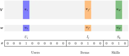
KTMs model the probability of observing binary out-comes of events (right or wrong), based on a sparse set of weights for all features involved in the event. Features in-volved in an event are encoded by a sparse vectorxof length

N such thatxi>0iff feature1≤i≤N is involved in the event. For each event involvingx, the probability p(x)to observe a positive outcome verifies:

ψ(p(x)) =µ+

N

∑

k=1

wkxk

  

logistic regression

+ ∑

1≤k<l≤N

xkxl⟨vk,vl⟩

  

pairwise interactions (1)

whereψis a link function such aslogit,µis a global bias, each feature i is modeled by both a biaswi ∈ R and an embeddingvi∈Rdfor some dimensiond. In what follows,

wwill refer to the vector of biases(w1, . . . , wN)andV to the matrix of embeddingsvi,i= 1, . . . , N. For each event,

only the features that have xi > 0 will contribute to the prediction, see Figure 1.

Data and Encoding of Side Information

We now describe how to encode the observed data in the learning platform into the sparse vectorx. First, we need to choose which features will be represented in the modeling.

Users Let us assume there arenstudents. The firstn fea-tures will be for alln students. As an example, if student

1≤i≤nis involved in the observation, itsxivalue will be set to 1, while the ones for the other students will be set to 0. This is called a one-hot vector.

Items Let us assume there aremquestions or items. One can allocatemmore features for allmquestions. If question

x w V

0 0 0 1 0 0 0 0 0 0 0 0 0 0 0 0 0 0

wi

vi

1

w_j0

vj0

1

wk0

vk0

U_i Ij Sk

Users Items Skills

Figure 1: Example of activation of a knowledge tracing ma-chine.

1≤j≤mis involved in the observation, its component in xwill be set to 1, while the ones for the other questions will be set to 0.

Skills We now assume there aresskills. We can then allo-catesextra features for thosesskills. The skills involved in an observation of a student over a questionjare the ones of

KC(j).

Attempts One can allocatesextra features as counters of how many opportunities a student could have learned a skill involved in the test.

Wins and Fails One can also distinguish between suc-cesses and failures: allocate sfeatures as opportunities to have learned a skill if the attempt was correct,smore fea-tures as opportunities to have learned a skill if the attempt was incorrect.

Extra side information More side information can be concatenated to the existing sparse features, such as the school ID and teacher ID of the student, or also other in-formation such as the type of test: low-stakes (practice) or high-stakes (posttest), etc.

Full example See Table 1 for an example of encoding of users + items + skills + wins + fails, for the set of ob-served, chronologically ordered triplets (2,2,1)(student 2 attempted question 2 and got it correct),(2,2,0),(2,2,1),

(2,3,0),(2,3,1),(1,2,1),(1,1,0). Here, we assume that there aren = 2students,m = 3questions, m = 3skills and question 1 does not involve any skill, question 2 in-volves skills 1 and 2, question 3 inin-volves skills 2 and 3. At the beginning, user 2 had no opportunity to learn any skill, so counters of wins and fails are all 0. After student 2 got question 2 correct, as it involved skills 1 and 2, the counters of wins for these two skills are incremented, and encoded for the next observation. We thus managed to encode the triplets withN =n+m+ 3s= 14features, and at training time, a bias and an embedding will be learned for each one of them.

Relation to Existing Models

Whenψ= logit, KTMs include IRT, AFM and PFA. Let us now recover some particular cases, especially whend= 0, i.e., only biases are learned for features, no embeddings. We will again assume there arenstudents,mquestions ands

skills.

We will note1i,na one-hot vector of sizen, which means all its components are 0 except theith one, which is 1.

Relation to IRT Ifd = 0, the second sum in Equation 1 disappears and all that is left is a weighted sum of biases.

If all features considered are students and questions (en-coding users + items), and we encode the pair (student i, questionj) as a concatenation of one-hot vectors1i,n and

1j,m, thenN =n+mandxk = 1iffk=iork=n+j. The expression in Equation 1 becomes:

log p(x)

(4)

Table 1: An example of encoding for training a knowledge tracing machine.

Users Items Skills Wins Fails

1 2 Q1 Q2 Q3 KC1 KC2 KC3 KC1 KC2 KC3 KC1 KC2 KC3

0 1 0 1 0 1 1 0 0 0 0 0 0 0

0 1 0 1 0 1 1 0 1 1 0 0 0 0

0 1 0 1 0 1 1 0 1 1 0 1 1 0

0 1 0 0 1 0 1 1 0 2 0 0 1 0

0 1 0 0 1 0 1 1 0 2 0 0 2 1

1 0 0 1 0 1 1 0 0 0 0 0 0 0

1 0 1 0 0 0 0 0 0 0 0 0 0 0

Outcome

1 0 1 0 1 1 0

Table 2: Datasets used for the experiments

Name Users Items Skills Skills per item Entries Sparsity (user, item) Attempts per user

Fraction 536 20 8 2.800 10720 0.000 1.000

TIMSS 757 23 13 1.652 17411 0.000 1.000

ECPE 2922 28 3 1.321 81816 0.000 1.000

Assistments 4217 26688 123 0.796 346860 0.997 1.014

Berkeley 1730 234 29 1.000 562201 0.269 1.901

Castor 58939 17 2 1.471 1001963 0.000 1.000

if the firstnfeatures (students numberediwhere1≤i≤n) have bias wi = θi −µ and the next m features (ques-tions numbered n + j where 1 ≤ j ≤ m) have bias

−dj. Therefore, KTM becomes after reparametrizationw=

(θ1−µ, . . . , θn−µ,−d1, . . . ,−dm)the 1-PL IRT model, also referred to as Rasch model.

Relation to AFM and PFA Now we will again consider the special cased = 0and an encoding of skills, wins and fails at skill level. For this, we will assume we know the Q-matrix, that is, the binary mapping between questions and skills(qjk)1≤j≤m,1≤k≤sas described in the introduction.

If we havew = (β1, . . . , βs, γ1, . . . , γs, δ1, . . . , δs)and encoding of “student i attempted questionj” is given by x= (qj1, . . . , qjs, qj1Wi1, . . . , qjsWis, qj1Fi1, . . . , qjsFis) whereWikandFik are the counters of successful and un-successful attempts at skill level, then KTM behaves like the PFA model. Similarly, one can recover the AFM model.

Relation to MIRT If d > 0, KTM becomes a MIRT model with user bias:

logitp(x) =θi−dj+⟨θi,dj⟩.

if the encoding is the same as for IRT (users + items with one-hot vectors). The reparametrization of weights is the same as for IRT, and the embeddings are given by V = (θ1, . . . ,θn,d1, . . . ,dm).

Training

Training of KTMs is made by minimizing the negative log-likelihoodN LLover allSobserved samples:

N LL(p(X),y) =

S

∑

i=1

yilogp(xi)+(1−yi) log(1−p(xi))

where we denote sample features byX = (xi)1≤i≤S and outcomes byy= (yi)1≤i≤S ∈ {0,1}S.

Like Rendle (2012), we assume some priors over the model parameters in order to guide training and avoid over-fitting.

Each bias wk follows wk ∼ N(µ,1/λ) and each em-bedding componentvkf, f = 1, . . . , dalso followsvkf ∼

N(µ,1/λ)whereµandλare regularization parameters that follow hyperpriorsµ∼ N(0,1)andλ∼Γ(1,1).

Because of those hyperpriors, we do not need to tune reg-ularization parameters by hand (Rendle 2012). As we use

ψ = probit, that is, the inverse of the CDF of the nor-mal distribution, we can fit the model using Gibbs sampling. Details of the computations can be found in (Freudenthaler, Schmidt-Thieme, and Rendle 2011).

The model is learned using the MCMC Gibbs sampler im-plementation of libFM2_{in C++ (Rendle 2012), using the} py-wFM Python wrapper3.

Visualizing the Embeddings

Another advantage of KTMs is that we can visualize the embeddings that they learn. On Figure 2, we show the 2-dimensional embeddings of users, items, skills learned by a knowledge tracing machine on the Fraction subtraction dataset. The user WALL·E is positively correlated with most of items, but not skills 2 (separate a whole number from a fraction) and 7 (substract numerators), which may explain why WALL·E couldn’t solve item 5 (4 3/5−3 4/10) that requires these two skills. Therefore, we can provide a useful feedback to WALL·E. To know more about the items and skills of this dataset, see (DeCarlo 2010).

2

http://libfm.org

3

(5)

0

1st component 0

2nd

comp

onen

t

1

2 3

4 5

6 7

8 9

10

11 12

13

14

15 16

17 18

19

20

1 2

3

4

5

6 7

8 WALL·E

item skill user

Figure 2: Example of learned 2-dimensional embeddings for the Fraction dataset.

Experiments

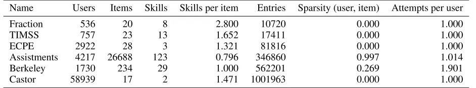
We used various datasets of different shapes and sizes in or-der to push our method to its limits. In Table 2, we report the main characteristics of the datasets: number of users, number of items, number of skills, average number of skills per item, total number of observed entries, sparsity of the (user, item) pairs, average number of attempts per user at item level.

Temporal Datasets

For the temporal datasets, students could attempt several times a same question, and potentially learn between at-tempts.

Assistments The 2009–2010 dataset of Assistments de-scribed in (Feng, Heffernan, and Koedinger 2009). 4217 stu-dents over 26688 questions, 123 KCs. 347k observations. There are many items but they involve 0 to 4 KCs, and there are only 146 combinations of KCs. For this dataset, we had also access to more side information, referred to as “extra” in the experiments:

• first action: attempt, or ask for a hint;

• school idwhere the problem was assigned;

• teacher idwho assigned the problem;

• tutor mode: tutor, test mode, pretest, or posttest.

Berkeley 1730 students from Berkeley attempting 234 questions from an online CS course, 29 KCs, exactly 1 KC per question, which is actually a category. 650k entries.

Non-Temporal Datasets

For all these datasets, the observations are fully specified: all users attempted all questions. All datasets except Castor can be found in the R package CDM (George et al. 2016).

Castor 58939 middle-school students over CS-related 17 tasks, 2 KCs, 1.47 KCs per task. 1M entries.

ECPE 2922 students over 28 language-related items, 3 KCs, 1.3 KCs per question in average. 81k entries.

0 100 200 300 400 500

Epochs 0.55

0.60 0.65 0.70 0.75

Accuracy

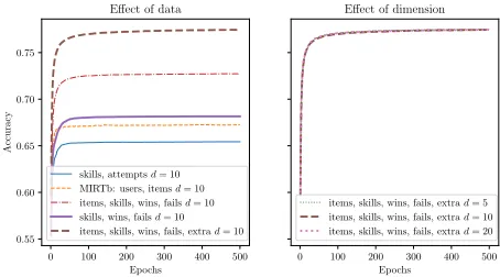
Effect of data

skills, attemptsd= 10 MIRTb: users, itemsd= 10 items, skills, wins, failsd= 10 skills, wins, failsd= 10 items, skills, wins, fails, extrad= 10

0 100 200 300 400 500

Epochs

Effect of dimension

items, skills, wins, fails, extrad= 5 items, skills, wins, fails, extrad= 10 items, skills, wins, fails, extrad= 20

Figure 3: Results for the Assistments dataset.

Fraction 536 middle-school students over 20 fraction sub-traction questions, 8 KCs, 2.8 KCs per question in average. 16k entries. A precise description of the items and skills is in (DeCarlo 2010).

TIMSS 757 students over 23 math questions from the TIMSS test in 2003, 13 KCs, 1.65 KCs per task. 17k entries.

Framework

From the triplets (user id,item id,outcome), we first compute for the temporal datasets the number of successful and unsuccessful attempts at skill level, according to the Q-matrix.

For each dataset, we perform 5-fold cross validation. For each fold, entries are separated into a train and test set, then we train different encodings of KTMs using the train set, no-tably the ones corresponding to existing models, and predict the outcomes in the test set.

KTMs are trained during 1000 epochs for each non-temporal dataset, 500 epochs for the Assistments dataset and 300 epochs for the Berkeley dataset, because it was enough for convergence. At each epoch, we average the results over all 5 folds, in terms of accuracy (ACC), area under the curve (AUC) and negative log-likelihood (NLL).

As special cases, as shown earlier, we have, for the tem-poral datasets:

• AFM is actually “skills, attemptsd= 0”

• PFA is actually “skills, wins, failsd= 0”

And for every dataset:

• IRT is “users, itemsd= 0”

• MIRT plus a user bias (coined as MIRTb) is “users, items” with anyd >0. Please note that for convenience, we used

probitinstead oflogitas link function for MIRTb.

Results and Discussion

(6)

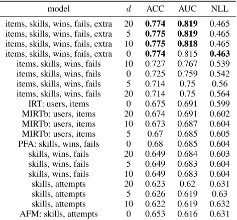
Table 3: Results for the Assistments dataset.

model d ACC AUC NLL

items, skills, wins, fails, extra 20 0.774 0.819 0.465

items, skills, wins, fails 10 0.727 0.767 0.539

IRT: users, items 0 0.675 0.691 0.599

MIRTb: users, items 20 0.674 0.691 0.602

PFA: skills, wins, fails 0 0.68 0.685 0.604

skills, wins, fails 20 0.649 0.684 0.603

skills, attempts 20 0.623 0.62 0.631

skills, attempts 5 0.626 0.619 0.63

skills, attempts 10 0.622 0.619 0.632

AFM: skills, attempts 0 0.653 0.616 0.631

Training Time

On the Assistments dataset, our model KTM(iswfe0) = “items, skills, fails, extrad = 0” is logistic regression, so it was faster to train (4 min 30 seconds on CPU for all 5 folds) than DKT (1 hour on CPU), while achieving higher AUC (0.815>0.743). For models of higher dimensions on this dataset, experiments took 17 min ford = 10with the same 31138 features, and 32 min ford= 20.

Effect of Side Information

Given its simplicity, IRT has a remarkable performance on all datasets considered, even on the temporal ones, which may be because the average number of attempts per stu-dent is small. When considering all information at hand, the top performing KTM model on the Assistments dataset ford= 0achieves higher performance than the known re-sults of vanilla DKT. It makes sense, as we have access to more side information, and logistic regression is less prone to overfitting.

Wins and Fails For all temporal datasets, encoding wins and fails (PFA model) instead of only the number of at-tempts (AFM model) improves the performance a lot (+0.07 AUC for Assistments, +0.01 for Berkeley). This is concor-dant with existing work (Pavlik, Cen, and Koedinger 2009). There is an improvement of KTM models that consider num-ber of wins and fails (KTM(iswf0) = “items, skills, wins, fails d = 0”) over IRT (+0.07 in Assistments, +0.02 in Berkeley).

Item Bias For all datasets, considering a bias per item im-proves the predictions, which is what IRT does but PFA does not. KTM(iswf0) = “items, skills, wins, fails d = 0” has

Table 4: Results for the Berkeley dataset.

model d ACC AUC NLL

IRT: users, items 0 0.688 0.753 0.586

PFA: skills, wins, fails 0 0.631 0.684 0.635

skills, attempts 20 0.621 0.675 0.639

AFM: skills, attempts 0 0.621 0.675 0.639

skills, attempts 10 0.621 0.675 0.639

skills, attempts 5 0.621 0.675 0.639

+0.07 AUC improvement over KTM(swf0) = PFA in Assist-ments, +0.09 in Berkeley. It may be because the number of items is huge, and they do not have the same difficulty. So, it is useful to learn this difficulty parameter using the per-formance of previous students. This extra parameter enables a big improvement on all datasets, except on the Fraction dataset, which may be because the skills for fraction subtrac-tion are easily known and clearly specified, so it is enough to characterize the items uniquely.

Skills For Fraction (8 KCs), Assistments (123 KCs) and TIMSS (13 KCs), the skills are easy to identify, because the items are math problems. For the other datasets, either there are few skills (ECPE: 3 language-learning KCs, Castor: 2 KCs for CS), or there is only one KC mapped to an item (Berkeley: 29 KCs, categories of CS problems). This is why considering a bias per skill barely increases the performance of the predictions.

Effect of Dimension of Features

On the temporal datasets, there is only a slight improvement of models with higher dimensions (less than +0.01 AUC), which seems to indicate that when there are many features considered (number of successful and unsuccessful attempts at item or skill level), a KTM with d = 0provides good enough predictions. Still, on a similar task, (Vie 2018) man-aged to get an improvement of +0.04 AUC for factoriza-tion machines ford = 20compared to logistic regression (d= 0), presumably because the side information was con-siderable for this task.

Further Work

(7)

Table 5: Summary of AUC results for all datasets.

AFM PFA IRT MIRTb10 MIRTb20 KTM(iswf0) KTM(iswf20) KTM(iswfe5)

Assistments 0.6163 0.6849 0.6908 0.6874 0.6907 0.7589 0.7502 0.8186 Berkeley 0.675 0.6839 0.7532 0.7521 0.7519 0.7753 0.7780 –

ECPE – – 0.6811 0.6807 0.6810 – – –

Fraction – – 0.6662 0.6653 0.6672 – – –

TIMSS – – 0.6946 0.6939 0.6932 – – –

Castor – – 0.7603 0.7602 0.7599 – – –

Side Information in Deep Knowledge Tracing

The vanilla DKT model cannot handle multiple skills, so instead, practictioners treat combinations of skills as new skills, which prevents the transfer of information between skills. The approach described in this paper can be used to handle multiple skills with DKT. Also, more recent results have successfully built upon the vanilla DKT (AUC 0.91>

0.743), by incorporating dynamic cluster information (Minn et al. 2018). We could indeed combine DKT with side infor-mation.

Adaptive Testing

IRT and MIRT were initially designed to provide adaptive testing: choose the best next question to present to a learner, given their previous answers. KTMs could also be used to these ends, as they extend the IRT and MIRT models with extra information, under the form of KCs or several at-tempts, and they maintain a measure of uncertainty though Bayesian inference.

Response Time, Spaced Repetition, and Other Data

Modeling response time could provide better predictions of outcomes, and it has also been used in the encoding of fac-torization machines in previous works. Also, we could add to the side information another counter representing how many timesteps were elapsed since a certain item was asked for the last time. It would learn how the user reacts to spaced repetition. In some datasets such as Assistments, more data is recorded about students that can be used to improve the predictions. Still, we should be careful about encoding noisy data such as the output of other machine-learning algorithms as side information, because it may degrade performance (Vie 2018).

Table 6: Results for the Fraction dataset.

model d ACC AUC NLL

MIRTb: users, items 20 0.619 0.667 0.651 items, skills 5 0.621 0.667 0.650 items, skills 20 0.621 0.666 0.649 MIRTb: users, items 5 0.621 0.666 0.650 IRT: users, items 0 0.623 0.666 0.656 users, items, skills 0 0.623 0.666 0.656 MIRTb: users, items 10 0.618 0.665 0.652 users, skills 5 0.62 0.664 0.649

Higher-Order Factorization Machines

In this paper, we were limited to pairwise interactions. But in his original paper (2012), Rendle mentions higher-order factorization machines, which generalize interactions tok -way terms. It could be an interesting direction for future research, as efficient methods have been developed to train these higher-order models (Blondel et al. 2016).

Ordinal Regression

Instead of binary outcomes, one could consider graded out-comes using multi-output FMs (Blondel et al. 2017) and thresholds, just like the graded response model in item re-sponse theory (Samejima 1997). We leave it to further work.

Conclusion

In this paper, we showed how knowledge tracing machines, a family of models that encompasses existing models in the EDM literature as special cases, could be used for the clas-sification problem of knowledge tracing.

We showed, using many datasets of various sizes and characteristics, that it could estimate user and item parame-ters even when the observations are sparse, and provide bet-ter predictions than existing models, including deep neural networks. KTMs are a testbed to try new combinations of data, such as response time, of number of attempts at item level.

One can refine the encoding of features in a KTM accord-ing to how the data was collected: Are the observations made at skill level or problem level? Does it make sense to count the number of attempts at item level or at skill level? What are extra sources of information that may raise better under-standing of the observations?

Furthermore, as we showed, KTMs are log-bilinear mod-els, so the embeddings they learn are interpretable, and can be used to provide useful feedback to students.

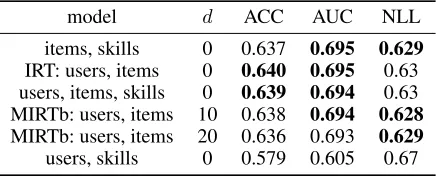
Table 7: Results for the TIMSS dataset.

model d ACC AUC NLL

(8)

Acknowledgments

We thank Florian Yger and the reviewers for their precious comments. We also thank Armando Fox and Nikunj Jain for providing the Berkeley dataset and Mathias Hiron for pro-viding the Castor dataset. Part of this research was discov-ered in a plane, so we also thank the flight attendants, that are always working hard to ensure our comfort.

References

Bergner, Y.; Dr¨oschler, S.; Kortemeyer, G.; Rayyan, S.; Seaton, D. T.; and Pritchard, D. E. 2012. Model-based collab-orative filtering analysis of student response data: Machine-learning item response theory. InProceedings of the 5th In-ternational Conference on Educational Data Mining, Chania, Greece, June 19-21, 2012, 95–102.

Blondel, M.; Fujino, A.; Ueda, N.; and Ishihata, M. 2016. Higher-order factorization machines. InAdvances in Neural Information Processing Systems, 3351–3359.

Blondel, M.; Niculae, V.; Otsuka, T.; and Ueda, N. 2017. Multi-output polynomial networks and factorization ma-chines. InAdvances in Neural Information Processing Sys-tems, 3349–3359.

Cen, H.; Koedinger, K.; and Junker, B. 2006. Learning fac-tors analysis–a general method for cognitive model evaluation and improvement. InInternational Conference on Intelligent Tutoring Systems, 164–175. Springer.

Cen, H.; Koedinger, K.; and Junker, B. 2008. Comparing two irt models for conjunctive skills. InInternational Conference on Intelligent Tutoring Systems, 796–798. Springer.

Corbett, A. T., and Anderson, J. R. 1994. Knowledge trac-ing: Modeling the acquisition of procedural knowledge.User Modeling and User-Adapted Interaction4(4):253–278. DeCarlo, L. T. 2010. On the analysis of fraction subtraction data: The DINA model, classification, latent class sizes, and the Q-matrix.Applied Psychological Measurement.

Desmarais, M. C., and Baker, R. S. 2012. A review of recent advances in learner and skill modeling in intelligent learning environments. User Modeling and User-Adapted Interaction

22(1-2):9–38.

Feng, M.; Heffernan, N.; and Koedinger, K. 2009. Addressing the assessment challenge with an online system that tutors as it assesses. User Modeling and User-Adapted Interaction

19(3):243–266.

Freudenthaler, C.; Schmidt-Thieme, L.; and Rendle, S. 2011. Bayesian factorization machines. Presented at the Work-shop on Sparse Representation and Low-rank Approximation, Neural Information Processing Systems (NIPS-WS).

George, A. C.; Robitzsch, A.; Kiefer, T.; Groß, J.; and ¨Unl¨u, A. 2016. The R package CDM for cognitive diagnosis mod-els.Journal of Statistical Software74(2):1–24.

Gonz´alez-Brenes, J.; Huang, Y.; and Brusilovsky, P. 2014. General features in knowledge tracing to model multiple sub-skills, temporal item response theory, and expert knowledge. In The 7th International Conference on Educational Data Mining, 84–91. University of Pittsburgh.

Lavou´e, E.; Monterrat, B.; Desmarais, M.; and George, S. 2018. Adaptive gamification for learning environments.IEEE Transactions on Learning Technologies1–12.

Minn, S.; Yu, Y.; Desmarais, M. C.; Zhu, F.; and Vie, J.-J. 2018. Deep knowledge tracing and dynamic student classi-fication for knowledge tracing. In2018 IEEE International Conference on Data Mining (ICDM), 1182–1187. IEEE. Pavlik, P. I.; Cen, H.; and Koedinger, K. R. 2009. Perfor-mance factors analysis–a new alternative to knowledge trac-ing. InProceedings of the 2009 conference on Artificial Intel-ligence in Education: Building Learning Systems that Care: From Knowledge Representation to Affective Modelling, 531– 538. IOS Press.

Piech, C.; Bassen, J.; Huang, J.; Ganguli, S.; Sahami, M.; Guibas, L. J.; and Sohl-Dickstein, J. 2015. Deep knowl-edge tracing. InAdvances in Neural Information Processing Systems (NIPS), 505–513.

Rendle, S. 2012. Factorization machines with libFM. ACM Transactions on Intelligent Systems and Technology (TIST)

3(3):57:1–57:22.

Samejima, F. 1997. Graded response model. InHandbook of Modern Item Response Theory. Springer. 85–100.

Sweeney, M.; Lester, J.; Rangwala, H.; and Johri, A. 2016. Next-term student performance prediction: A recommender systems approach. JEDM — Journal of Educational Data Mining8(1):22–51.

Thai-Nghe, N.; Drumond, L.; Horv´ath, T.; Krohn-Grimberghe, A.; Nanopoulos, A.; and Schmidt-Thieme, L. 2011. Factorization techniques for predicting student performance. Educational recommender systems and technologies: Practices and challenges129–153.

Thai-Nghe, N.; Drumond, L.; Horv´ath, T.; and Schmidt-Thieme, L. 2012. Using factorization machines for student modeling. InProceedings of FactMod 2012 at the 20th Con-ference on User Modeling, Adaptation, and Personalization (UMAP 2012).

Vie, J.-J. 2018. Deep factorization machines for knowledge tracing. In Proceedings of the Thirteenth Workshop on In-novative Use of NLP for Building Educational Applications, 370–373.

Wilson, K. H.; Karklin, Y.; Han, B.; and Ekanadham, C. 2016a. Back to the basics: Bayesian extensions of IRT out-perform neural networks for proficiency estimation. In Pro-ceedings of the 9th International Conference on Educational Data Mining (EDM), 539–544.

Wilson, K. H.; Xiong, X.; Khajah, M.; Lindsey, R. V.; Zhao, S.; Karklin, Y.; Van Inwegen, E. G.; Han, B.; Ekanadham, C.; Beck, J. E.; et al. 2016b. Estimating student proficiency: Deep learning is not the panacea. Presented at the Workshop on Machine Learning for Education, Neural Information Pro-cessing Systems.