www.adv-radio-sci.net/11/23/2013/ doi:10.5194/ars-11-23-2013
© Author(s) 2013. CC Attribution 3.0 License.
Radio Science
Eigenvalue extraction from time domain computations
T. Banova1,2, W. Ackermann2, and T. Weiland2
1Technische Universit¨at Darmstadt, Graduate School of Computational Engineering, Dolivostraße 15, 64293 Darmstadt,
Germany
2Technische Universit¨at Darmstadt, Institut f¨ur Theorie Elektromagnetischer Felder (TEMF), Schlossgartenstraße 8,
64289 Darmstadt, Germany
Correspondence to: T. Banova ([email protected])
Abstract. In this paper we address a fast approach for an accurate eigenfrequency extraction, taken into consideration the evaluated electric field computations in time domain of a superconducting resonant structure. Upon excitation of the cavity, the electric field intensity is recorded at different detection probes inside the cavity. Thereafter, we perform Fourier analysis of the recorded signals and by means of fit-ting techniques with the theoretical cavity response model (in support of the applied excitation) we extract the requested eigenfrequencies by finding the optimal model parameters in least square sense. The major challenges posed by our work are: first, the ability of the approach to tackle the large scale eigenvalue problem and second, the capability to ex-tract many, i.e. order of thousands, eigenfrequencies for the considered cavity. At this point, we demonstrate that the pro-posed approach is able to extract many eigenfrequencies of a closed resonator in a relatively short time. In addition to the need to ensure a high precision of the calculated eigen-frequencies, we compare them side by side with the refer-ence data available from CEM3D eigenmode solver. Further-more, the simulations have shown high accuracy of this tech-nique and good agreement with the reference data. Finally, all of the results indicate that the suggested technique can be used for precise extraction of many eigenfrequencies based on time domain field computations.
1 Introduction
The field of quantum chaos encompasses the study of the manifestations of classical chaos in the properties of the corresponding quantum or more generally, wave-dynamical system (nuclei, atoms, quantum dots, and electromagnetic or acoustic resonators). Prototypes are billiards of arbitrary shape. In its interior a point-like particle moves freely and
is reflected specularly at the boundaries. Depending on the shape its properties could exhibit chaotic dynamics.
Within this work, we investigate quantum billiards with its statistical eigenvalue properties, which reveal the periodic orbits in the quantum spectra and give the quantum chaotic scattering (Dembowski et al., 2005). Specifically, we sim-ulate microwave resonator with chaotic characteristics, see Fig. 1, and we compute the eigenfrequencies that are needed for its level spacing analysis (Dembowski et al., 2002). Ac-cordingly, the eigenfrequency level spacing analysis for de-termining the statistical properties requires many (in order of thousands) eigenfrequencies to be calculated and the accu-rate determination of the eigenfrequencies has a crucial sig-nificance. Moreover, considering that the problem is to com-pute a large number of eigenfrequencies, they can be often located in different ranges, i.e. left-most, right-most or inte-rior portions of the spectrum could be sought.
In many scientific and engineering applications, as well as, in computational science, this results in solving one of the fundamental problems, the large scale eigenvalue prob-lem. We list below just a few of the applications areas (Saad, 2011) where eigenvalue calculations arise: acceler-ation of charged particles, structural dynamics, electrical networks, Markov chain techniques, combustion processes, chemical reactions, macro-economics, control theory, etc. The above-mentioned realistic applications frequently chlenge the limit of both computer hardware and numerical al-gorithms, as the involved matrices are of large scale.
24 T. Banova et al.: Eigenvalue extraction from TD computations
challenge from our application is that the dimension of the desired eigen subspace is large, namely, one might possibly need thousands of eigen pairs located in a specified range, also referred to as a “window”, of matrices with dimension in excess of several millions. Despite the fact that many algorithms for eigenvalue determination exist, accompanied by the numerical models that are becoming increasingly more sophisticated, not as many are specifically adapted for computing a large number of interior eigen pairs. They can usually calculate limited number of extreme or interior eigenfrequencies, and relatively few are designed for effec-tively reusing a large number of good initial presumptions, when they are available. Finally, computing a large number of interior eigenvalues remains one of the most difficult problems in computational linear algebra today.
In this context, our investigations comprise efficient, ro-bust and accurate computations of many desired eigenfre-quencies in a reasonable time, which also constitutes the main aim of our study. Within this work, we cover an ap-proach for extraction of resonant frequencies given the out-put from time domain comout-putations of closed resonators. The proposed approach uses the advantage that one single time domain simulation can provide the whole response of an electromagnetic system in a wide frequency band, whereas a frequency domain formulation uses one computation for each individual frequency. In addition, due to the fact that the time domain computations in the field of electromagnet-ics are already highly developed and considerably more ef-ficient, as well as the fact that the transient solver contained in CST Microwave Studio (CST, 2012) uses a high degree of parallelization provided with modern graphics processing units (GPUs) feature the simulation can be dramatically ac-celerated. Therefore, we can easily and quickly get the time domain responses for a wide frequency band. In this way, sig-nificant reduction in computation time can be achieved and therefore, our high interest leads to time domain computa-tions for electromagnetic problems.
The paper proceeds as follows. In Sect. 2 we briefly present the proposed approach for high precision eigenfre-quency extraction given the available electric field computa-tions. Here, we describe the fundamental modeling of the an-alyzed structure, followed by a description of the used signal postprocessing techniques. Section 3 investigates the simula-tion scenarios together with the obtained results. Lastly, con-clusions are addressed in Sect. 4.
2 Time domain approach for eigenfrequency extraction This section provides a brief overview of a precise time-domain (TD) approach for eigenfrequency extraction, which is applicable for different cavity structures. In a two-step pro-cess the modeling and simulation of a specific cavity struc-ture is initially done, and afterward a postprocessing of the acquired time domain simulation results in MATLAB
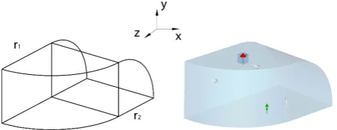
(MAT-Fig. 1. Left: desymmetrized version of the three-dimensional
gener-alized stadium billiard, consisted of two quarter cylinders with radii r1=200.0 mm andr2=141.4 mm. Right: CST setup of the
bil-liard cavity with an exciting antenna and detection probes placed at various positions.
LAB, 2011) is conducted. A descriptive sketch of the pro-posed TD approach is given in Algorithm 1. Additionally, the critical implementation points and details are covered, as well as, discussed within this section.
2.1 Field simulation in time domain
The proposed approach for eigenfrequency extraction (given in the following) is utilized within the project for determin-ing the statistical properties of a cavity with chaotic char-acteristics. The requirements for chaotic characteristics are met by using a superconducting resonator with the shape of a desymmetrized three-dimensional stadium billiard (see Fig. 1-left). The billiard consists of two quarter cylinders with radii r1=200.0 mm andr2=141.4 mm, respectively,
and is made of niobium, which becomes superconducting at temperatures below 9.2 K.
The cavity of interest is modeled in CST Microwave Stu-dio (CST MWS) and a small tiny exciting antenna (as used in a physical model) is put properly in a way that the modes within a specific frequency range would be excited (see Fig. 1-right). Intentionally, the excitation signal applied at the antenna input is wide band signal, i.e. a Gaussian-modulated sinusoidal signal is chosen, which certainly covers the range of eigenfrequencies being sought. The field simulation with hexahedron discretization mesh in time domain is carried out with the transient solver from CST MWS and it detects and records the electric field intensity at specific field detection probes placed at various positions inside the cavity (see lines 1–6 in Algorithm 1). Later, the obtained time domain sig-nals are used for further postprocessing in MATLAB, based on fitting techniques with a proposed model of the cavity re-sponse, as follows below.
2.2 Postprocessing of the CST signals 2.2.1 Limitations from finite simulation time
T. Banova et al.: Eigenvalue extraction from TD computations 25
0 0.5 1 1.5 2
x 10−7 −5000
0 5000
a) Time/s
E−field Probe
1.4 1.45 1.5 1.55 1.6 x 10¹⁰ 0 50 100 150 b) Frequency/Hz Amplitude
1.495 1.5 1.505
x 1010 50
100 150
c) Frequency/Hz
Amplitude
TD signal TD signal * Gausswin
0 5 10 15
x 10−8 −100
0 100
d) Time/s Amplitude spectrum
Gaussian pulse Gaussian modulated signal
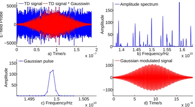
Fig. 2. Operating signals during the process of eigenfrequency extraction, listed in the respective sub-figures. (a) Acquired time domain
signal and Gaussian windowed time domain signal. (b) Amplitude spectrum of the Gaussian windowed time domain signal. (c) Isolated Gaussian pulse within the eigenmode spectrum. (d) Gaussian modulated signal.
0 0.5 1 1.5 2
x 10−7 −5000
0 5000
a) Time/s
E−field Probe
1.4 1.45 1.5 1.55 1.6 x 10¹⁰ 0 50 100 150 b) Frequency/Hz Amplitude
1.495 1.5 1.505
x 1010 50
100 150
c) Frequency/Hz
Amplitude
TD signal TD signal * Gausswin
0 5 10 15
x 10−8 −100
0 100
d) Time/s Amplitude spectrum
Gaussian pulse Gaussian modulated signal
Fig. 2.Operating signals during the process of eigenfrequency extraction, listed in the respective sub-figures. a) Acquired time domain signal and Gaussian windowed time domain signal. b) Amplitude spectrum of the Gaussian windowed time domain signal. c) Isolated Gaussian pulse within the eigenmode spectrum. d) Gaussian modulated signal.
Input: Given a cavity with a specified probeP(x,y,z).
/* CST simulation */
Data: run transient simulation with the predefined simulation
time.
Data: export aT D sigfor the electric field intensity in
P(x,y,z).
/* Post processing and frequency
extraction in MATLAB */
T D sig=T D sig∗gausswin(size(T D sig)); f f t data= fft(T D sig);
amp spec= abs(f f t data);
forall theGaussian pulses inamp specdo
gauss pulse= locate gauss pulse();
/* ind start=starting index
ind end=ending index */
GoF1 = cftool(gauss pulse,gauss model());
/* GoF = Goodness of Fitting */
ifGoF10then
gausswin f f t data(ind start:ind end) =
f f t data∗gausswin(ind end−ind start);
forall theind /∈gauss pulsedo
gausswin f f t data(ind) = 0;
end
gauss mod sig= real(ifft(gausswin f f t data));
GoF2 =
cftool(gauss mod sig,gauss mod model());
ifGoF2'100then
extract the eigenfrequency;
end end end
Algorithm 1: A sketch of the time domain approach for
extracting eigenfrequencies.
the power losses in the walls are negligible. Theoretically, the response of an ideal-conducting cavity is Dirac impulse sequence in frequency domain, i.e. a summation of sinu-soidal signals with the associated eigenfrequencies in time domain. Nevertheless, due to the limited simulated time
160
interval the ideal Dirac impulses of the true spectrum are widened. Moreover, due to the finite conductivity and the in-serted antenna, the amplitude spectrum of the signal does not contain Dirac delta pulses, but it has pulses of finite width.
An important issue coming from the limitation in time is
165
the discontinuities at the edges of the measured time (Mandal and Asif, 2010). Given that sharp discontinuities have broad frequency spectra, these will lead to a higher side lobes level and each spectral line of the signal’s frequency spectrum will be spread out in the same way. In other words, the spreading
170
means that signal energy, which should be concentrated only at one eigenfrequency, leaks instead into other frequencies, the so called ’spectral leakage’. Consequently, the whole spectrum is distorted and some weak impulses, i.e., eigen-frequencies, can be masked by the resulting convolution with
175
neighboring strong pulses. This leads to the idea of multiply-ing the original signal within the measurement time by Gaus-sian function (see Fig. 2a) that smoothly reduces the signal to zero at the end points of the measurement time: therefore avoiding discontinuities overall (see line 9 in Algorithm 1).
180
As a result, in case of an ideal cavity, whose spectrum theo-retically is constituted of Dirac impulses located at the eigen-frequencies, we would have Gaussian pulses instead (see Fig. 2b).
Furthermore, manifestation of a spectral distortion occurs
185
as result of a reduced spectral resolution. Namely, this is an important issue, and the minimum separation needed
be-the power losses in be-the walls are negligible. Theoretically, be-the response of an ideal-conducting cavity is Dirac impulse se-quence in frequency domain, i.e. a summation of sinusoidal signals with the associated eigenfrequencies in time domain. Nevertheless, due to the limited simulated time interval the ideal Dirac impulses of the true spectrum are widened. More-over, due to the finite conductivity and the inserted antenna, the amplitude spectrum of the signal does not contain Dirac delta pulses, but it has pulses of finite width.
An important issue coming from the limitation in time is the discontinuities at the edges of the measured time (Mandal and Asif, 2010). Given that sharp discontinuities have broad frequency spectra, these will lead to a higher side lobes level and each spectral line of the signal’s frequency spectrum will be spread out in the same way. In other words, the spreading means that signal energy, which should be concentrated only at one eigenfrequency, leaks instead into other frequencies, the so called “spectral leakage”. Consequently, the whole spectrum is distorted and some weak impulses, i.e., eigenfre-quencies, can be masked by the resulting convolution with neighboring strong pulses. This leads to the idea of multi-plying the original signal within the measurement time by Gaussian function (see Fig. 2a) that smoothly reduces the signal to zero at the end points of the measurement time: therefore avoiding discontinuities overall (see line 9 in Algo-rithm 1). As a result, in case of an ideal cavity, whose spec-trum theoretically is constituted of Dirac impulses located at the eigenfrequencies, we would have Gaussian pulses instead (see Fig. 2b).
26 T. Banova et al.: Eigenvalue extraction from TD computations
that they can be resolved. In our approach, we choose the frequency resolution good enough to recover the sought fre-quency data. As a result, a large number of simulation time samples might be needed for a reliable characterization of the resonance frequency of the structure, given that better frequency resolution unescapably requires a longer simula-tion time. In spite of this, the modern GPUs feature a large number of processing cores and the simulation is speeded up significantly in comparison with a simulation running on sin-gle CPU.
2.2.2 Fast Fourier transformation
As soon as the limitations that come from finite simulation time or reduced frequency resolution are overcame, the step from the recorded time domain response to the frequency do-main response is computed using the fast Fourier transforma-tion (see lines 10–11 in Algorithm 1, see Fig. 2b).
The very classical approach in finding eigenfrequencies is to look for local maxima of the eigenmode spectrum. How-ever, this way is not efficient when the interest is in pre-cise determination of the resonant frequencies and has some drawbacks. Firstly, the spectrum is discrete with a certain res-olution and the peak value may not be entirely located on a sample point. The eigenfrequency could be a value that is somewhere in the range between two samples given with the frequency resolution for certain discrete frequency val-ues (“bins”), implying that the local maximum is not always the frequency that is sought. Secondly, a more serious focus was placed that the neighboring modes contribute a certain amount to the total response at the resonance of the mode being analyzed and affect slightly the resonant frequency. To deal with these problems, refined modal extraction methods based on signal processing techniques have been developed (see lines 12–31 in Algorithm 1).
2.2.3 Technique for locating a Gaussian pulse
For further analysis, local Gaussian pulses (see Fig. 2c) within the spectrum should be located properly (see line 13 in Algorithm 1). The location process is divided into several steps. Primarily, a local Gaussian pulse is found as a set of samples with a local maximum. Thereafter, supplementary check is conducted if some other samples might be added to the right-most/left-most side of the current Gaussian pulse. Namely, if the average amplitude of the succeeding right/left outer triple of samples is less than the average amplitude of the right-most/left-most triple of samples, the outer triple of samples is added appropriately to the right/left part of the Gaussian pulse. After that, the “empirical rule” for the cur-rent located Gaussian pulse is applied. For this purpose, the standard deviation for the pulse is estimated and four stan-dard deviations are accounted for the resulting pulse. At the end, the distance from the both ends of the Gaussian pulse to its maximum is equally adjusted.
2.2.4 Fitting models
By invoking the acquired knowledge of the eigenmode spec-trum of the cavity, the fitting model should be nonlinear in the parameters, i.e. we should use Gaussian nonlinear model to obtain the parameters. In this direction, the parametric fit-ting is involved as essential technique for precise determina-tion of the eigenfrequencies and reducing the amount of data required for a given resolution. Relying on the above discus-sion, a custom Gaussian model is modeled within the MAT-LAB curve fitting tool (see line 16 in Algorithm 1), which suits to the specific curve fitting needs, as shown below:
yi =ai
−(f−fi )2
2σi2 , (1)
wherei goes from unity to the number of the located local Gaussian pulses in the amplitude spectrum for the analyzed structure. With this model all of the local Gaussian pulses are fitted and in eachi-th fitting the values for the found param-etersai,fi, andσi are saved. The parametersai andfi are
used as initial reasonable starting values of the parameters in the further fit, whereas the parameterσi is included to
in-crease the numerical robustness. The values of the parameter fi are good candidates for eigenfrequencies, since they give
the position of the maximum value of each Gaussian pulse. However, following this way we are restricted to a limited number of samples, same as the number of samples which constitute the local Gaussian pulse. The limitation in the sam-ples causes that the coefficient, which represents the good-ness of fitting, is very low. That means that the accuracy of the eventual eigenfrequency cannot be high. Additionally, with this approach only the amplitude information of the sig-nal is used, which is not sufficient for precise extraction.
These disadvantages lead to extending our approach, in a sense where we can get also the phase information of the signal in a form that is suitable for implementation. Namely, after fitting a local Gaussian pulse in frequency domain the values of the parameters and the coefficients for the good-ness of the fit are obtained. If the goodgood-ness of the fit for some Gaussian pulse is positive then we window this Gaus-sian pulse with GausGaus-sian windowing function and we go back in time domain using Inverse Fast Fourier Transform (IFFT) (see lines 18–31 in Algorithm 1). Otherwise, we do not take into consideration this pulse, which is most probably noise. From signal processing is known that shifting in frequency domain means modulation in time domain. So, the Gaussian-modulated sinusoidal signalyi=aisin(2πfit−φi)
−(t−t0)2
2σi2
is expected in time domain. The frequency of the modulation fi is exactly the frequency that is sought. Consequently, we
The main advantage comparing the proposed approach with the classical approach for finding the peaks, is that within this approach the phase information of the signal is used and parametric fitting with all of the data available in the time domain representation is applied. Although, the fit-ting based only on the amplitude information of the signal results in poor fit, now using the phase information of the signal, very good value for the goodness of the fit can be reached. In this way, as shown in Sect. 3, we gain a very high accuracy in the eigenfrequency extraction from time domain computations.
2.2.5 Nonlinear parametric fitting
The fitting process uses the method of nonlinear least squares, presented in Nash and Sofer (1996) and Lewis et al. (2006), which minimizes the summed square of residuals, identified as error associated with the data, given by
S=
n X
i=1
ri2=
n X
i=1
(yi− ˆyi)2, (2)
where the residualri for thei-th data point is defined as the
difference between the observed response valueyi and the
fitted response valueyˆi whilenis the number of data points
included in the fit. In case of nonlinear models the parame-ters cannot be estimated using simple matrix techniques and these models are particularly sensitive to the starting points. This leads to difficult fit and the starting points are adjusted. Therefore, at the beginning initial reasonable starting values for each parameter are provided. Then, the iterative approach follows some steps until the fit reaches the specified conver-gence criteria. At the end, the direction and magnitude of the adjustment of the parameters depends on the Levenberg-Marquardt fitting algorithm proposed by Levenberg (1944), Marquardt (1963), and Mor´e (1978).
3 Simulation results
The accuracy of the TD method for eigenfrequency ex-traction is tested for both analytically and non-analytically resolvable problems. Additionally, the proper functionality of the method has been checked during its implementation process. In the numerical tests, several resonators are con-sidered. Namely, due to verification purposes, rectangular, cylindrical and spherical resonant structures are analyzed, whose exact solution can be analytically evaluated. Firstly, the eigenvalues of the above mentioned resonators are com-puted from their analytical expressions and following this way, a logarithmic relative error is calculated as
relative error=log10
fanalytical−fnumerical
fanalytical
, (3)
by considering the first computed mode eigenfrequency, un-less otherwise stated.
Besides the analytically resolvable resonators, the rela-tive error is also measured for the chaotic billiard resonator, which has a clustered eigenvalue distribution (Dembowski et al., 2002). A clustered distribution containing too close eigenfrequencies might cause difficulties in the eigenfre-quency extraction. As reference data, eigenvalues calculated with CEM3D eigenmode solver for different degrees of free-dom (DOF) are computed. Here, CEM3D eigenmode solver is a parallel program, developed by (Ackermann and Wei-land, 2012) for the accurate calculations of eigenfrequencies for a given structure. It implements a FEM formulation by means of higher order curvilinear elements.
In all simulations, we first modeled and meshed the re-lated geometries in CST MWS with hexahedrons and saved the electric field intensity during the transient simulation. Af-terward, the eigenvalue extraction is calculated in MATLAB. In the simulation studies, we experienced that for the time domain field computations, a single personal computer is suited for problems with a moderate number of degrees of freedom (say, up to 106DOF). To be precise, a computer with a single core Pentium 3 GHz processor and 6 GB main mem-ory was used. The same PC configuration was also utilized for the TD method for eigenvalue extraction. On the other hand, a more powerful computer was necessarily used to en-able the handling of meshes with hundreds of thousands up to several millions DOF. The larger-scale simulations were performed on a GPU computer, e.g. 2.00 GHz (quadcore) having 32 GB RAM memory and 4 nVIDIA Quadro GPUs. 3.1 Rectangular, cylindrical, and spherical cavity As a first experiment, we consider a rectangular cavity with perfectly conducting walls, containing a perfect vacuum. The degeneracy is broken by making the side lengths different, i.e. rectangular resonator with dimensions a=20 cm, b= 10ecm, and c=10πcm. The resonance frequency of the rectangular microwave cavity for the TE011mode (the mode
with the lowest cutoff frequency for a rectangular waveg-uide wherec > b > a) is found by imposing boundary condi-tions on the electromagnetic field expressions in which all of the field components vary sinusoidally at a single frequency (Pozar, 1998).
Along this line, the fundamental mode in a cylindrical cav-ity (Reitz and Milford, 1960) with radius R=20 cm and lengthL=10πcm is calculated, too. For the analyzed cylin-drical cavity, since we do not have large L fulfilling L > 2.03R, the TM010 mode constitutes the fundamental
oscil-lation. The mode of interest has azimuthal symmetry and the electric field has no longitudinal variation (δE/δz=0).
Lastly, the first TM101mode of a spherical resonator with
28 T. Banova et al.: Eigenvalue extraction from TD computations
0.005 0.01 0.02 −5 0.05 0.1 0.2 0.5 1 2 5
−4.5 −4 −3.5 −3 −2.5 −2
Hexahedral meshcells/Million
lo
g10
--
-ˆf−
f
f
--
-Rectangular cavity (1st mode)
Cylindrical cavity (1st mode)
Spherical cavity (1st mode)
O(log10(cells)−2/3)
Fig. 3. Relative deviation of the numerically obtained valuesfˆfor the lowest eigenfrequency to the analytical resultf as a function of the degrees of freedom (DOF) for a rectangular, cylindrical, and spherical resonator.
Specifically, for the time domain field simulations several different discretization meshes have been used and the con-vergence study based on the calculation of a relative error, given with Eq. (3), is shown in Fig. 3. As the number of dis-cretization mesh cells increases, the difference between the analytical and the numerical solutions becomes smaller and absolute error in order of 10−4 is present. So, fast conver-gence is observable and it should be emphasized. As sug-gested by the convergence study, good accordance of the nu-merical with the analytical results is evident.
3.2 Billiard cavity
Using the previosly described algorithm, about 900 eigenfre-quencies up to 7 GHz have been calculated for the billiard cavity structure. Unfortunately, for this shape of resonator an analytical solution for the electromagnetic problem is not available and in order to validate the obtained results, ref-erence data from CEM3D eigenmode solver are used (see Fig. 4). The structures are modeled and meshed with curvi-linear tetrahedrons and the corresponding meshes are im-ported to CEM3D eigenvalue solver in order to compute the requested eigenfrequencies for the analyzed structure.
In Fig. 4, a part of the results that are found with the TD approach compared to the reference data, is presented. On the abscissa are given the frequencies in an a priori se-lected frequency band, i.e. from 1.8 up to 2.4 GHz. The ordinate shows the eigenfrequencies obtained with the time domain approach using four different discretization meshes, and the reference data calculated using a field simulation in frequency domain with two different tetrahedral meshes. The total time for the transient simulations is 3.5×10⁻⁵s, which results in frequency resolution of 30 kHz.
The results in Fig. 4 indicate that when fine mesh is used the number of eigenfrequencies found with the proposed TD approach is exactly the same as the reference data, i.e. no ad-ditional frequency is added or no missed. In addition, such check was conducted for all of the 900 calculated
eigen-Cells: 59,292
Cells: 461,214
Cells: 3,882,816
Cells: 23,356,890
Tets: 318,425
1.8 1.9 2 2.1 2.2 2.3 2.4
x 109
Frequency/Hz Tets: 7,056
Fig. 4. Convergence study showing a comparison between the
eigenfrequencies calculated with the proposed TD approach (red color) and the reference eigenfrequencies obtained with CEM3D eigenmode solver based on higher order curvilinear elements (green color). For the TD approach four different hexahedron discretiza-tion meshes are used. At the same time, the reference data are ob-tained using two different tetrahedral discretization meshes.
Cells: 59,292
Cells: 461,214
Cells: 3,882,816
Cells: 23,356,890
Tets: 5,568,907
Tets: 318,425
2.3 2.31 2.32 2.33 2.34 2.35 2.36 2.37
x 109
Frequency/Hz Tets: 7,056
Fig. 5. Convergence study showing a comparison between the
eigenfrequencies calculated with the proposed TD approach (red color) and the reference eigenfrequencies obtained with CEM3D eigenmode solver based on higher order curvilinear elements (green and blue color). For the TD approach four different hexahedron dis-cretization meshes are used. At the same time, the reference data are obtained using three different tetrahedral discretization meshes.
0.02 0.05 0.1 0.2 0.5 1 2 5 10 20 50 −4.5
−4 −3.5 −3 −2.5
Hexahedral meshcells/Million
lo
g10
--
-ˆf−
f
f
--
-Mode 2.36 GHz Mode 2.37 GHz
O(log10(cells)−2/3)
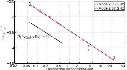
Fig. 6. Relative deviation of the numerically obtained valuesfˆto the reference results f as a function of the degrees of freedom (DOF) for a billiard resonator. Two eigenfrequencies are consid-ered: 2.36 GHz and 2.37 GHz mode eigenfrequency.
approach can be used for precise extraction of eigenfrequen-cies from time domain computations.
4 Conclusions
In conclusion, we have presented an approach for eigenfre-quency extraction when the time domain response for a su-perconducting closed resonator is available and when plenty of eigenfrequencies are required. The approach is relatively fast and very simple compared to others presented in litera-ture. In addition, we have inspected the robustness and con-vergence of the proposed technique in time domain with the reference data determined by the CEM3D eigenmode solver with higher order curvilinear elements. Hereby, the conclu-sion shows that the proposed approach results in solutions which agree well with the reference data, gaining high accu-racy and efficiency in eigenvalue extraction. Finally, all of the results indicate that the proposed TD technique can be used in different areas of applications, where a precise extraction of plenty of eigenfrequencies takes a crucial role.
Acknowledgements. The work of Todorka Banova is supported by the “Excellence Initiative” of the German Federal and State Gov-ernments and the Graduate School of Computational Engineering at Technische Universit¨at Darmstadt.
References
Ackermann, W. and Weiland, T.: High Precision Cavity Simula-tions, Proceedings of the 11th International Computational Ac-celerator Physics Conference, 1–5, 2012.
CST AG, CST 2012, Darmstadt, Germany, MICROWAVE STU-DIO, 2012.
Dembowski, C., Dietz, B., Gr¨af, H.D., Heine, A., Papenbrock, T., Richter, A., and Richter, C.: Experimental Test of a Trace For-mula for a Chaotic Three Dimensional Microwave Cavity, Phys. Rev. Lett., 89, 064101, doi:10.1103/PhysRevLett.89.064101, 2002.
Dembowski, C., Dietz, B., Friedrich, T., Gr¨af, H.D., Harney, H.L., Heine, A., Miski-Oglu, M., and Richter, A.: Dis-tribution of resonance strengths in microwave billiards of mixed and chaotic dynamics, Phys. Rev. E, 71, 046202, doi:10.1103/PhysRevE.71.046202, 2005.
Gallagher, S. and Gallagher, W. J.: The Spherical Resonator, IEEE Trans. on Nuclear Sci. Vol NS-32 5, 1985.
Mandal, M. and Asif, A.: Continuous and Discrete Time Signals and Systems, Posts & Telecom Press, 2010.
Marquardt, D.: An Algorithm for Least Squares Estimation of Non-linear Parameters, SIAM J. Appl. Math, 11, 431–441, 1963. MATLAB R2011b, The MathWorks Inc., Natick, MA, 2011. Mor´e, J. J.: The Levenberg-Marquardt Algorithm: Implementation
and Theory, Lecture Notes in Mathematics, v630, edited by: Wat-son, G., Springer, 1978.
Nash, S. G. and Sofer, A.: Linear and Nonlinear Programming, McGraw-Hill Companies, Inc, New York, ISBN 0-07-046065-5, 1996.
Levenberg, K.: A Method for the Solution of Certain Problems in Least Squares, Quart. Appl. Math, 2, 164–168, 1944.
Lewis, J. M., Lakshmivarahan, S., and Dhall, S.: Dynamic Data As-similation: A Least Squares Approach (Encyclopedia of Mathe-matics and its Applications), Cambridge University Press, 2006. Pozar, D. M.: Microwave Engineering, 2nd edition, John Wiley and
Sons, Inc., New York, NY, 1998.
Reitz, J. R. and Milford, F. J.: Foundations of Electromagnetic The-ory, Addison-Wesley, 1960.