Coda wave interferometry during the heating of deep geothermal reservoir rocks

Coda wave interferometry

during the heating of deep geothermal

reservoir rocks

Jérôme Azzola

_{, Luke Griffiths}

_{, Jean Schmittbuhl}

_{, Dimitri Zigone}

_{, Vincent Magnenet}

_{, Frédéric Masson}

_,

Michael Heap

_{and Patrick Baud}

Abstract

Coda wave interferometry (CWI) is a high-resolution technique that aims at tracking small changes in a diffusive medium from the time correlation of seismic waveforms. CWI has been widely used in recent years to monitor the fine-scale evolution of fault zones and more recently of deep reservoirs. However, to provide a quantitative interpretation of the reservoir, direct modeling of physical effects like the influence of temperature on seismic wave scattering is required to investigate temperature effects from measurements of velocity changes. Here, we propose to quantify the impact of thermo-elastic deformation on CWI measurements by comparing experimental results obtained from a previous study on Westerly Granite to a numerical approach based on two combined codes (SPECFEM2D and Code_Aster) for modeling wave propagation in complex media during thermo-elastic deformation. We obtain two major results. First, we show that multiple reflections on the boundaries of our simplified numerical sample reproduce well the wave scattering properties of the experimental granitic sample characterized by a complex mineral assembly and a large set of microcracks. We based our comparison on the wave diffusion model that describes both the experi-mental and numerical samples (similarity in energy density function and mean free path). We also show that both samples share a similar thermo-elastic behavior, but only after the second heating and cooling cycle. Second, the stretching technique used for CWI measurements on both samples reveals reversible time shifts correlated with the thermo-elastic deformation of the sample. However, the influence of thermo-elastic deformation is different between our numerical proxy and the experimental sample. We discuss the role of irreversible deformation (e.g., microcracking) for the observed discrepancy by introducing temperature dependence of elastic moduli in the model. These results suggest that there are open perspectives to monitor thermal strain in geothermal reservoirs using CWI.

Keywords: Coda wave interferometry, Westerly Granite, Deep geothermal reservoir, Wave propagation simulation (SPECFEM2D), Thermo-elastic deformation simulation (Code ASTER)

Open Access

© The Author(s) 2018. This article is distributed under the terms of the Creative Commons Attribution 4.0 International License (http://creat iveco mmons .org/licen ses/by/4.0/), which permits unrestricted use, distribution, and reproduction in any medium, provided you give appropriate credit to the original author(s) and the source, provide a link to the Creative Commons license, and indicate if changes were made.

RESEARCH

Background

At the laboratory scale, seismic methods, both active (ultrasonic wave velocity meas-urements) and passive (acoustic emission monitoring), provide a range of monitoring techniques to analyze the influence of temperature on a rock sample. In particular, coda wave interferometry (CWI) is a method that has recently been used to monitor ther-mal microcracking in granite (Griffiths et  al. 2018). CWI uses scattered elastic waves observed in the late part of the seismogram (i.e., the coda) to track small changes in solid materials such as rocks (e.g., Poupinet et  al. 1984; Ratdomopurbo and Poupinet 1995; Roberts et al. 1992; Snieder 2002). The late arrivals are indeed much more sensi-tive to small-scale perturbations as they intensively sample the medium through multi-ple scattering which leads to diffusive waves and equipartition (e.g., Ryzhik et al. 1996; Weaver 1982; Hennino et  al. 2001; Snieder 2006). Crystals present in a granitic rock sample, for example, not only play a specific role in the thermal microcracking, but also act as many distinct scatterers, contributing to the diffusion of the wavefield propagat-ing within the sample. This method is appropriate to follow both reversible phenomena such as elastic deformation, and irreversible phenomena such as thermo-elastic effects, which deeply impact the propagation of elastic waves and can thus be studied using late arrivals in the coda. For example, Grêt et al. (2006) used CWI on an Elberton Granite sample heated to 90 °C to measure the influence of temperature changes on ultrasonic wave velocity. They interpreted the arrival time perturbations measured in the coda of strongly scattered waves recorded while heating as an apparent decrease in wave veloc-ity. This drop in apparent velocity presents a strong non-linear behavior when the sam-ple was heated from 70 to 90 °C, occurring contemporaneously with an increase in the acoustic emission rate, attributed to thermal microcracking. Consistent changes in rock microstructure have been recently monitored within a wider range of temperatures in Westerly Granite using the same CWI method (Griffiths et al. 2018). Westerly Granite is an interesting material for laboratory experiments as it has been extensively studied (e.g., Brace et al. 1966, 1968) and its physical properties are well known. The fine crystal size of Westerly Granite, about 1 mm in diameter, is similar to the so-called “two-mica granite” (e.g., Hooijkaas et al. 2006) which hosts the deep geothermal reservoir exploited at the Enhanced Geothermal System (EGS) test site in Soultz-sous-Forêts, France. Com-bining velocity measurements, acoustic emission monitoring, and high-resolution CWI measurements within a new experimental setup, Griffiths et  al. (2018) monitored the microstructural evolution of Westerly Granite during multiple heating cycles from room temperature to 450 °C. Interestingly, the study highlighted different mechanical behav-iors between the first and the subsequent cycles. While large and mostly permanent changes in the waveforms were measured during the first cycle, interpreted as an appar-ent reduction in velocity with temperature, the reductions in wave velocity during the following cycles were lower in amplitude (Griffiths et al. 2018).

Chaki et al. 2008; Meredith et al. 2012). The influence of temperature variations on these mechanical parameters is more complex to understand when the rock sample is cycli-cally heated and cooled. This situation is, however, relevant for thermally dynamic envi-ronments such as geothermal reservoirs (e.g., sequences of mud circulations in wells during drilling, thermal stimulation of the wells, variations in well flow during exploita-tion, etc.). Indeed, the impact on the mechanical properties and characteristics of the rock may vary from one cycle to another. For instance, Thirumalai and Demou (1974) measured the thermal dilatation of two granites (Halecrest and Charcoal Granite) dur-ing cyclical heatdur-ing and cooldur-ing. They observed a permanent dilatation of the granites following the first cycle, but the dilatation during the third cycle was reversible. During the first heating/cooling cycle, their observations show that microcracking occurred in the sample. The following cycles had a much-reduced impact on microcracking.

Understanding the influence of temperature changes on the physical and mechanical properties of reservoir rocks is an important issue for the monitoring of deep geother-mal reservoirs such as Enhanced Geothergeother-mal Systems (EGS) (Olasolo et  al. 2016; Lu 2018). One of the most representative rocks of the EGS reservoirs of the Upper Rhine Graben is granite. For example, at the Soultz-sous-Forêts site (France) (Gérard and Kap-pelmeyer 1987; Gérard et al. 2006), a fractured granitic reservoir (Genter and Traineau 1996; Dezayes et al. 2005; Hooijkaas et al. 2006; Ledésert et al. 2010; Villeneuve et al. 2018) is overlain by a 1.5 km-thick sedimentary unit (Aichholzer et al. 2016; Griffiths et al. 2016; Heap et al. 2017; Kushnir et al. 2018a, b). The crystals and mineral inclusions in granite also play a specific role in its thermal response. Indeed, heating of a granitic rock results in the complex thermal expansion of its various minerals and leads to the build-up of thermal stresses that may induce thermal microcracking (Kranz 1983; Fre-drich and Wong 1986; Griffiths et al. 2018). At a larger scale, thermal stimulation can promote the fracturing of a rock mass (Huenges and Ledru 2011). The increase in frac-turing due to thermal stimulation will increase the permeability (e.g., Siratovich et al. 2015), and ultimately the efficiency, of the geothermal system. As the physical properties of rock are non-trivially influenced—at all scales—by changes in temperature and pres-sure, laboratory experiments on representative granite rock samples and the forward modeling of the involved processes are necessary to develop relevant seismic monitoring techniques and help to improve geothermal optimization.

contributions of various physical processes (velocity changes, heterogeneity of the elas-tic deformation field, amplitude variations, etc.) on CWI measurements. The modeling approach of Azzola et al. (2018) combined a spectral element approach (SPECFEM2D) to study the seismic wave propagation within a diffusive medium, while elastic deforma-tion of the medium was modeled using a finite element code (Code_Aster) (Azzola et al. 2018).

We analyze the wave propagation properties of a medium that reproduce both acousti-cally and mechaniacousti-cally the measurements on the Westerly Granite rock sample during heating from room temperature to 450 °C, with a specific focus on its thermo-elastic deformation. CWI of synthetic waveforms generated while heating or cooling are com-pared to laboratory measurements (Griffiths et al. 2018). The first section describes the principle of the methods developed in both studies. As a framework for the numerical modeling, the experimental method of Griffiths et al. (2018) is detailed first, as well as the experimental evolution of the waveforms during heating and cooling. The numeri-cal scheme that models the experiment is presented as well as the principle of CWI in this methodology section. In “Results”, results of the comparison of the experimental and numerical approaches are given for the wave scattering properties and the thermo-mechanical behavior of the samples. We then show the CWI signals measured at the laboratory and in the simulation, as a function of the sample temperature. The differ-ences in behavior are discussed in “Results” on the basis of the dependence of mechani-cal parameters with temperature. Finally, conclusions are proposed in “Conclusions”.

Methods

Summary of the experimental approach used by Griffiths et al. (2018) Laboratory sample description

Figure 1a presents the experimental apparatus used to measure changes in ultrasonic wave velocity during repeated heating and cooling cycles of a cylindrical sample (20 mm diameter and 40 mm length) of Westerly Granite (from Rhode Island, USA). Westerly Granite was chosen as it is well-studied, and its physical and mechanical properties are well known and are near-isotropic (Lockner 1998). Furthermore, the physical, mechani-cal, and transport properties of Westerly Granite have been shown to exhibit permanent changes related to thermal microcracking when heated to temperatures of above 70 °C (Nasseri et al. 2007, 2009; Wang et al. 1989; Yong and Wang 1980; Griffiths et al. 2018).

Laboratory setup description

The rock sample was held between two vertical pistons made of heat resistant stainless steel (grade 310) and loaded using a LoadTrac II servo-controlled uniaxial press (Fig. 1a). A tube furnace with a constant temperature zone of 80 mm surrounded the sample. Fur-ther details of the experimental setup are provided in Griffiths et al. (2018).

of diameter 1.5 mm inserted through a 1.7 mm hole drilled radially to the center of the sample.

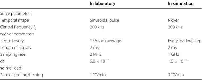
During the thermal stressing of the sample, a pair of high temperature sensors used for acoustic measurements were in direct contact with opposing faces of the sam-ple, as presented in Fig. 1a. The pair of acoustic sensors are considered as broadband, since they have a weak resonant frequency at 100  kHz and an operating frequency range of 80–560 kHz. Using a signal generator, a 200 kHz sinusoidal pulse was emit-ted every 50  ms at the upper transducer (source). The generator simultaneously trig-gered an acquisition card to record the pre-amplified voltage signal at the receiver (the lower transducer). 2 ms duration waveforms were recorded at a sampling rate of 2 MHz. Table 1 summarizes the parameters of the source receiver used in the setup. To ensure a constant coupling between the sensors and the sample during heating and cooling, both transducers were held in direct contact on the opposing faces of the granite sample using an axially applied force of 100 N, equating to a uniaxial stress of approximately 0.3 MPa on a 20 mm diameter sample.

Under ambient temperature conditions, measurements of the P-wave velocity, vP, and S-wave velocity, vS, were performed using a separate, calibrated apparatus prior to, and following all three heating/cooling cycles using first arrivals (contrary to late arrivals in the coda for CWI). These measurements provided a reference for the velocity measure-ments. Measurements were made using two pairs of piezo-transducers in contact with

Silent air-cooling system 44 kN Load Cell

Cylindrical rock sample Steel upper piston

Thermal insulation

LoadTrac II uniaxial press

Tube furnace

High temperature resistant broadband acoustic sensors

a

b

20 40 60 80

Experiment time (hours)

0 100 200 300 400

Sample temperature (°C)

0

Fig. 1 a Sketch of the experimental setup (modified from Griffiths et al. 2018) for wave velocity

opposing faces of the samples. One pair was oriented parallel to the sample length to measure P-wave first arrival times. The other, oriented perpendicular to the sample length, provided S-wave first arrival times. The source function was a sinusoidal pulse: 700 kHz for P-wave, and within the range 100–500 kHz for S-wave velocity.

Numerical modeling of the experiment Physical properties of the sample

Our numerical simulations described below in “Results” intend to reproduce the experi-mental setup of Griffiths et al. (2018). The goal of the numerical analysis is to gain insight into the influence of temperature variation on the seismic wave velocity of granite. Our numerical approach focuses on the contribution, in the thermo-elastic domain, of reversible deformation. We also consider additional simulations designed to study the influence of temperature, a factor that greatly influences density, Young’s modulus and bulk modulus, on the CWI measurements.

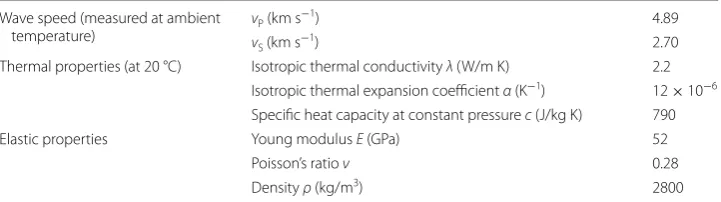
One of the main issues of the numerical approach is to introduce a numerical sam-ple that accurately reproduces the macroscopic mechanical behavior of the real granite sample, as well as its wave diffusion properties while remaining as simple and homoge-neous as possible. The dimensions of the numerical sample were chosen to be of same as the experimental sample (40 × 20  mm). From wave velocity measurements carried out on the intact sample of Westerly Granite, at ambient temperature, we estimate mac-roscopic Poisson’s ratio ν and to define P and S-wave velocities, respectively, noted vP and vS. Young’s modulus E, density ρ and the thermal properties of the rock (isotropic thermal conductivity λ—thermal dilatation coefficient α—specific heat capacity c) are chosen from Heard and Page (1982), Maqsood et al. (2004), Park et al. (2004), Dwivedi et al. (2008) and Schön (2011) to depict Westerly Granite. Measurements and mechani-cal parameters are presented in Table 2.

The wavelength used in the experimental work means that most of the scattering comes from multiple reflections on the boundaries of the sample, rather than reflections from crystal boundaries (Griffiths et al. 2018). This wave scattering behavior is repro-duced in the numerical sample as we do not include details of the crystal assembly, but only use the multiple reflections at the free boundaries of the sample.

Table 1 Parameters of the sensors and source function used in the laboratory experiments (S9215 high temperature sensors from  Physical Acoustics) and  in  the simulation with heating and cooling rates

In laboratory In simulation

Source parameters

Temporal shape Sinusoidal pulse Ricker

Central frequency f₀ 200 kHz 200 kHz

Receiver parameters

Record every 17.5 s on average Every loading step

Length of signals 2 ms 2 ms

Sampling rate 2 MHz 1 GHz

dt 5.0 × 10−7 _{1.0 × 10}−9

Thermal load

The waveform recorded at a given receiver in the simulation is subsequently the con-tribution of many reflected waves that have travelled along multiple paths through the sample. The numerical sample is discretized using a 2D finite element mesh grid of 17244 elements with a characteristic length lc = 0.5 mm. This parameter corresponds to the characteristic distance between two neighboring nodes. The meshing of the sample is done using GMSH which is a GNU General Public License finite element mesh gen-erator with 2-D quadrangle meshes using a Delaunay algorithm.

Numerical scheme description

The numerical simulation relies on combining two codes. The iterative thermo-mechan-ical deformation of the mesh grid is first obtained using the finite element software

Code_Aster (EDF R&D, general code for the study of the mechanical behavior of the structures). Each step of the loading process consists of the resolution of a linear thermal problem, which is combined to a mechanical loading that takes into account the 0.3 MPa axial stress applied to the cored sample (Griffiths et al. 2018). We first solve the thermal problem according to the following equation:

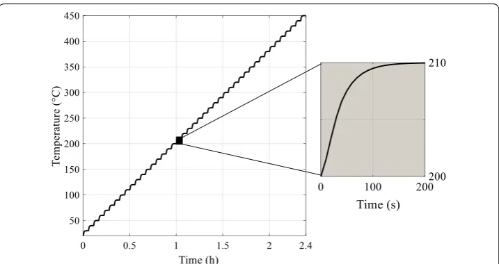
Temperature conduction within the sample is treated as an evolutionary regime. Fig-ure 2 shows the evolution of temperature with simulation time computed by Code_Aster

at the center of the sample. The insert on the right of Fig. 2 details the evolution during one step of the thermal deformation of the sample, when temperature is increased by 10 °C from 200 to 210 °C. For each thermal step, the initial state is a homogeneous tem-perature field T=Ti, and the thermal loading is an imposed temperature on the edges of the sample T=Ti+ 10 °C. The insert of Fig. 2 shows how temperature diffuses with time during a given loading step and shows that the stabilization time is about 100 s. It also shows that the temperature field is homogenous to 10−3 _{°C following 200 s, which} justi-fies the initialization of each thermal step by a homogeneous field. This heating rate (of about 3 °C/min; Table 1) is necessary for the stabilization of temperature at the end of each step of the simulation, in line with the quasi-thermal equilibrium in the laboratory experiments (heating rate of 1 °C/min; Table 1).

(1)

(ρ·c)·dT/dt+ div

−·grad(T)

= 0.

Table 2 Elastic and  thermal parameters of  the  medium of  the  simulation used in Code_ Aster and  SPECFEM2D to  reproduce the  mechanical and  acoustic behavior of  the  cored sample used in the experiments

Young’s modulus, density and the thermal properties of the rock are chosen from Heard and Page (1982), Maqsood et al. (2004), Park et al. (2004), Dwivedi et al. (2008) and Schön (2011)

Wave speed (measured at ambient

temperature) vP (km s

−1_{) 4.89}

v_S (km s−1_{) 2.70}

Thermal properties (at 20 °C) Isotropic thermal conductivity λ (W/m K) 2.2 Isotropic thermal expansion coefficient α (K−1_{) 12 × 10}−6 Specific heat capacity at constant pressure c (J/kg K) 790

Elastic properties Young modulus E (GPa) 52

Poisson’s ratio ν 0.28

Equation (1) includes a dependency of the density with the temperature. We first recall that density is directly related to the volumetric deformation evol:

Second, S-wave speed v and density ρ are linked by

where K is the bulk modulus and E is the Young’s modulus, are assumed constant in the simulation, in the thermo-elastic domain. As a consequence, a volumetric change of the medium during heating or cooling results in an increase in density, and subsequently in a velocity change. To discuss this influence of the medium density changes on the CWI measurements, the variation of relative time delays with volumetric strain are analyzed in “Results”.

The numerical scheme is based on the chaining of a thermal and a mechanical prob-lem. As a result, we solve the mechanical problem according to the following equation:

with C the elasticity tensor, α the thermal dilatation, etot the total deformation, T and Ti the temperature and reference temperature of 25 °C. We neglect the effects of gravity in Eq. (2). The calculations carried out with Code_Aster result in a displacement field at the nodes of each element. At each step, the current mesh grid is then deformed accordingly to the computed displacement field.

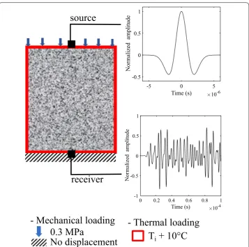
The updated mesh grid is then an input of SPECFEM2D (a 2D spectral element code; see Komatitsch and Vilotte 1998). It simulates the wave propagation in the medium from the emitted source assuming free boundaries. A Ricker Wavelet of dominant frequency f0= 200 kHz (see top-right inset of Fig. 3) is sent in the medium (2) evol=δVol/Vol0= −δρ/ρ0.

(3) v=3·K·E/ρ·(9·K−E),

(4) div [C(etot−α·(T− Ti))]=0,

from the source and recorded at the opposite side by a 32-sensor long receiver line (see bottom-right insert of Fig. 3 for an example of recorded seismogram at a given receiver position). Absolute locations of the sources and receivers remain unchanged from the onset to the end of the deformation process. Table 1 details the parame-ters of the source–receiver pairs used in both the laboratory and in the simulation. The numerical approach that we developed allows us to test the effect of the elastic deformation of the sample independently of intrinsic wave velocity variations. When focusing in a first approach on the influence of reversible deformation in the thermo-elastic domain, wave velocities in all elements are kept constant. The only parame-ter evolving during successive steps is the mesh grid. In laboratory experiments, the effects of reversible elastic deformation are in general difficult to distinguish from intrinsic variations that are related to anelastic and irreversible processes like damage

-5 0 5

Time (s) ₁₀-6

-0.5 0 0.5 1

Normalized amplitude

0 0.2 0.4 0.6 0.8 1 -1

-0.5 0

Time (s) ₁₀-4 0.5

1

- Mechanical loading

0.3 MPa

No displacement

- Thermal loading

Normalized amplitude

T

+ 10°C

source

receiver

development (Snieder 2006). In a second approach, bulk and Young’s modulus, den-sity and thereby elastic wave velocities depend on temperature, which enables us to discuss the partitioning between each effect. The flexibility of the numerical approach complements the laboratory experiments and compensate for its limits.

In the following sections, the “reference” seismogram refers to the one recorded at ambient temperature T=T0, and the “perturbed” seismogram refers to the one recorded at a given temperature. CWI is used to compare these perturbed seismograms with the “reference” one to analyze changes induced by the thermo-elastic deformation.

Coda wave interferometry (CWI)

Coda wave interferometry aims to track small velocity changes in solid materials, such as rocks, where elastic waves are strongly diffused. As a result of the strong diffusion, coda waves intensively sample the medium through multiple scattering, such that the travel time delays measured between “reference” and “perturbed” waveform taken in the coda are much more sensitive to slight perturbations in the medium than in the early part of the waveform (e.g., Poupinet et al. 1984; Snieder 2006; Campillo and Roux 2015). Changes occurring in the medium—which include structural changes, the displacement of scatterers or mechanical deformation of the boundaries—delay the travel time of these scattered waves (Stehly et al. 2007), which make them observable using stretching or correlation methods.

Description of the coda wave interferometry techniques

The CWI measurements performed in the laboratory and in the simulation are based on a stretching approach of the whole signal, the first arrivals being a negligible part of the signal. Sens-Schönfelder and Wegler (2006) proposed to estimate the relative time differences ε= δt/t in the late part of the signal between two successive acquired wave-forms, as the factor by which the time axis of one of the traces must be stretched or compressed to obtain the best correlation with the other trace. In this technique, one defines “stretched” versions of one of the waveform of the pair such as S(t) =R((1 +a)t), with a given coefficient of stretching a. Following Sens-Schönfelder and Wegler (2006) and Larose and Hall (2009), we use a spline interpolation in the time domain to stretch the waveform. We then calculate the cross-correlation function between the other unstretched waveform of the pair with several stretched waveforms. The relative time shift—i.e., the relative variation of delay with time, assuming a linear variation of the delays in the coda—is equal to the value of a corresponding to the maximum of the cross-correlation function. This method is applied to the first 0.5 ms of the seismograms.

Application to laboratory and numerical results

The significant perturbation of the medium during the thermal loading induces a sig-nificant evolution of the waveforms and leads to a weak correlation between the first recorded waveform, the reference, and subsequent waveforms recorded during heating. Accordingly, it is not possible to apply the stretching technique using the first waveform as a unique reference. As a result, the waveform recorded at a given temperature T=Tk

relative time shift ε(Ti, T0) is obtained from the comparison of the waveform recorded at a given temperature Ti, with respect to the reference waveform, recorded at temperature T0, according to Eq. (5), from a scaling factor and the preceding relative time shifts ε(Tk, Tk− 1):

In the numerical simulation, waveforms are compared in pairs using a stretching approach along the 2 ms long signal (Sens-Schönfelder and Wegler 2006). Since the sim-ulated waveforms are weakly perturbed by the thermal loading, they are all compared to the initial waveform (not incrementally as in the experiments). We verified that the incremental comparison of pairs of simulated waveforms and their comparison to a common reference led to identical CWI results.

The receiver line used in the numerical modeling is a 32-sensor long array. Seismo-grams are thus acquired on distinctive receivers equally distributed along the bottom of the sample for each wave propagation modeling. This specificity of the numerical model enables us to analyze the spatial variability of our numerical measurements, given that CWI methods are applied at each receiver. When comparing a given pair of waveforms by stretching, we calculate the dispersion of the 32 distinctive relative time shifts esti-mations as well as the mean relative time shift. The fluctuations in the measurements are minor: the standard deviation of this population typically represents 8% of the mean value. It demonstrates the spatial homogenization occurring in our sample due to the diffraction of the wavefield. As a result of this spatial homogenization, the relative time shift measured in our numerical approach at each step of the thermal loading of the sample is the average of the 32 distinctive estimations.

Results

Comparison of the wave scattering properties

We check here that the numerical sample reproduces the acoustic behavior of the gran-ite sample used in the laboratory experiments. For this, we compare the scattering prop-erties of the numerical sample and the granite sample, by computing the energy density

W(r, t) for both the experimental and numerical records in the same manner as Wegler and Lühr (2001) according to the following equation:

Here, fi (in m s−1), for i varying from 1 to 3, are the components of the

seismo-gram measured in the simulation and in the laboratory experiments at ambient tem-perature. H is the Hilbert transform. The observed energy density function is then compared to the wave diffusion model for body waves. This allows us to estimate the mean free path l by least square fitting, as proposed in Olivier et al. (2015). The mean free path is the mean distance between two consecutive diffusion events and is a key parameter to assess the development of the diffusive wavefield in both propagation (5) ε(Tk,T0)=

k

i=1

(ε(Ti,Ti−1)+1)−1.

(6) W(r,t)=

3

i=1

f_i2+H(fi)2

media. As shown in Nakamura (1977) and Dainty and Toksöz (1977, 1981), the dif-fusion model predicts the seismic energy of multi-scattered body waves W(r, t) as a function of time and space:

where W(r, t) is the energy density, Es the source energy, vS the S-wave velocity, r the distance to the source, ηi the intrinsic attenuation defined as the inverse of the intrinsic absorption characteristic length la and ηs the scatter attenuation which is the inverse of the mean free path l. Equation (7) is linearized by choosing an adequate reference in time t1 and distance r1 so that W1(r1, t1) = 1 J m−3, and by taking the natural logarithm of a referenced function U(t) defined in Eq. (8). Three dimensionless coefficients a1, a2 and a3 appear in Eq. (8) and are expressed with parameters of the model (Wegler and Lühr 2001):

It appears that a3 is expressed as a function of the intrinsic attenuation. Intrinsic attenuation is the inverse of the mean free path, which enables us to estimate the mean free path from a3:

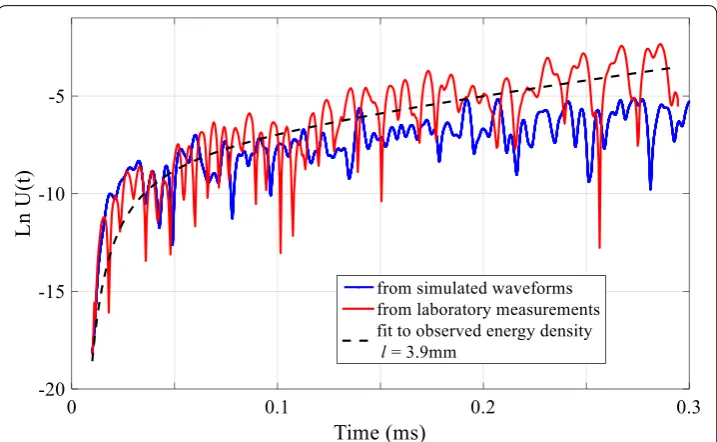
The observed energy density function W(r, t) is linearized by multiplying Eq.  (3) with the geometric factor t3/2 _{and by taking the natural logarithm of both sides, which} allows us to reconstruct the left side of Eq. (8). Figure 4 shows the logarithmic repre-sentation of the energy density functions computed with the first 0.3 ms of the origi-nal waveforms recorded at the laboratory and in the simulation. The comparison of these functions shows that the numerical medium used in the simulation describes the wave scattering occurring in the experimental granite sample. The comparison presented in Fig. 4 shows that a longer time is required to obtain a diffuse wavefield in the medium than in the real granite sample. Grain inclusions that contribute to diffuse the wavefield in addition to the multiple reflections in the real granite sample could explain this difference in behavior.

Dimensionless coefficients a1, a2 and a3 are estimated using a least square fitting from Eq. (8). With vS= 2700 m s−1 and r= 40 mm, we finally estimate the mean free path using Eq. (9). Figure 4 shows in addition the model obtained by a least square (7) W(r,t)=Es·

4·π·vs·t

3·ηs −3₂

·e

−ηi·vs·t−

3·r2·ηs

4·vs·t

,

(8) LnU(t)=a1+a2·t+

a3

t .

with U(t)=

W(r,t) W1 · t t1 3₂

and a1=ln

E0 W1

·4·π·vs·t1 (3·ηs)

−3₂

; a2=ηi·vs; a3= −

3·ηs·r2 4·vs .

fitting of the linearized energy density functions Ln U(t) computed from the labora-tory results. The mean free path is estimated to be l= 3.9 mm.

The application of CWI techniques requires the strong scattering regime to be estab-lished. In multi-scattering regimes, the wave front emitted from the source sees the heterogeneities several times before reaching the receiver. The condition necessary to assess strong scattering is that the mean free path l, the size of the defects d, the size of sample D (here, 40 mm), and the wavelength λ are satisfying the inequality: λ≤d≤l≤D

(Planès and Larose 2013). In our setup, we calculated a mean free path l= 3.9 mm. The

wavelength λ= 12  mm is estimated using the central frequency of the Ricker source and the S-wave velocity. This shows that the inequality and the requirements for strong scattering are not satisfied. Meanwhile, both linearized energy density functions exhibit strong similarities: the medium of the simulation properly describes the scattering that occurred in the experimental sample. To fulfill the condition of strong scattering, the laboratory experiments and the simulation would have required a source of higher fre-quency. To gain insight on the consequences of not verifying the inequality on the sim-ulated and laboratory CWI results, we ran simulations with a Ricker source of higher frequencies: f0= 800 kHz and up to f0= 1000 kHz. In each of these simulations, the cal-culated wavelength (respectively, λ= 3 mm and λ= 2.4 mm) and the revalued mean free path satisfy the condition for strong scattering. With f0= 800 kHz, the model obtained by least square fitting corresponds to an estimated mean free path l= 5.6 mm and with

f0= 1000 kHz, it is l= 5.3 mm.

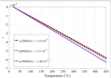
Figure 5 shows the simulated CWI measurements obtained for the three central fre-quencies as well as the linear regressions fitted to the measurements. It shows that the

slope of the linear regression at higher frequencies s(f0= 800 kHz) and s(f0= 1000 kHz) present less than 5% of variations compared with the reference s(f0= 200 kHz). This test demonstrates that, even if the inequality for strong scattering is not perfectly fulfilled for

f0= 200 kHz, it is possible to extract relevant information from the diffuse wavefield at that central frequency.

Comparison of the mechanical behavior

The numerical sample intends to reproduce the mechanical behavior of the granite sam-ple used in the laboratory experiments. In the simulation, we focus on the elastic defor-mation of the sample when the temperature is progressively increased from 20 to 450 °C in 10 °C increments. The mesh grid, which is an input for the wave propagation simula-tion, is progressively deformed. As the mechanical parameters are considered constant with temperature, the numerical scheme intends to test the effect of the material defor-mation (in particular of thermal dilatation of the sample), independent of intrinsic per-turbations related to inelastic deformation (microcracks, plastic deformation, etc.).

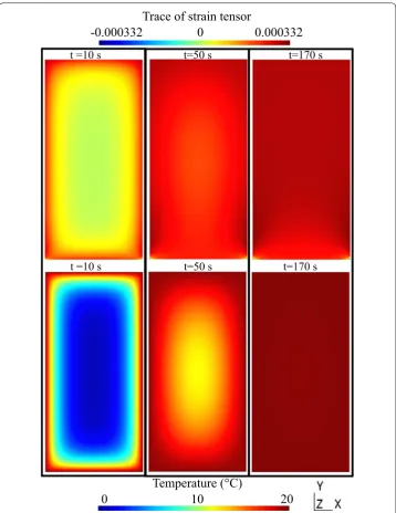
The volumetric deformation is computed as the trace of strain tensor (obtained from

Code_Aster): volumetric strain evol is the sum of the components eYY and eXX of the strain tensor. Figure 6 shows three maps of the volumetric deformation, at the beginning of the heating process (t= 10 s), while temperature diffuses (t= 50 s) and after stabilization of

the temperature (t= 170 s), in the simulation. Each map of the volumetric deformation

(top panels in Fig. 6) is associated with the corresponding map of the temperature field Fig. 5 Comparison of simulated CWI measurements obtained for three different central frequencies

(bottom panels). The temperature, recorded at the center of the sample each time a 10 °C increment is set at its boundaries, is also represented in Fig. 3.

The temporal evolution of the temperature field shows the progressive diffusion of heat within the sample, from the moment the boundary conditions are applied at the boundaries of the sample to the homogenization of the temperature field. The tempera-ture field and the volumetric deformation stabilize after about 100 s. This duration is consistent with the characteristic time of diffusion τ=e2_{/D computed from the} charac-teristic length of diffusion e and the thermal diffusivity D. According to the parameters

Trace of strain tensor

-0.000332 0 0.000332

Temperature (°C)

0 10 20

t =10 s t=50 s t=170 s

chosen in Table 2, D=λ/ρ·c= 10.0 × 10−7 _m2 _s−1_{. Considering the size of the sample} (40 × 20  mm) and the temperature increase imposed at its boundaries, we calculate

τ= 100 s.

Maps generated following the stabilization of the temperature field (170 s) show the homogeneity of the sample deformation. At the bottom of the sample, the strain field is influenced by the specific mechanical boundary condition of the bottom, which is fixed without any horizontal or vertical displacement.

Results obtained in the laboratory, unlike in the simulation, show that permanent changes in microstructure occur with temperature. As the sample is heated for the first time, a high acoustic emission (AE) rate is contemporaneous with large—and mostly per-manent—apparent reductions in velocity with temperature (Griffiths et al. 2018). P-wave velocity is reduced by 50% of the initial value at 450 °C, and 40% upon cooling: the rela-tive time shift is posirela-tive during heating and negarela-tive during cooling and a net apparent decrease in velocity of 17% is highlighted following the first cycle. Griffiths et al. (2018) observed fewer permanent changes in wave velocity during the second heating/cooling cycle, and less again during the third cycle. During these two cycles, the change in veloc-ity was reversible: the velocveloc-ity decreased by roughly 10% of its initial value when the sample was heated to 450 °C and increased again during cooling. Griffiths et al. (2018) attributed the reversible velocity increase/decrease to the elastic expansion/contraction of crystals, and the associated opening/closing of microcracks.

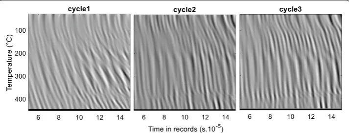
To illustrate this variability of behavior during the cycles of the experiments, the three panels of Fig. 7 show zooms of the waveforms, from 50 to 150 µs. The 100 µs long wave-forms recorded during the first, second and third heating of the sample are stacked. The horizontal axis indicates time in the coda, the vertical axis the sample temperature, the gray level the waveform amplitude. Figure 7 first illustrates the “stretching” effect, show-ing that the arrival times of the scattered waves appear shifted towards later arrival times when the sample temperature rises. The waveform looks like physically stretched when the temperature increases (in opposition to the compression of the waveforms observed during cooling) and the CWI method applied intends to quantify the relative variation of time delays with time, ε= δt/t. The comparison between the three panels shows then

that the amplitude of this stretching phenomenon is different between the first and

subsequent cycles. Indeed, it shows that the amplitude of the relative time delay—with reference to the waveform recorded at ambient temperature—increases significantly from 180  °C, which is not the case during the second and third cycles for which the stretching of the waveforms is more linear with temperature and of similar amplitude. Figure 7 highlights that the irreversible non-linear changes linked to thermal microc-racking dominate during the first cycle (Griffiths et  al. 2018), but are reduced during subsequent cycles, which are instead dominated by the thermo-elastic deformation of the sample. We compare in the following the simulated CWI measurements to those recorded during the second or third cycle in the laboratory such that the numerical model describes the physics of the experiment.

CWI results

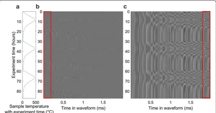
In Fig. 8, we stacked the original waveforms recorded during three heating and cooling cycles, for both the laboratory measurements and the simulation. It enables us to com-pare the numerical response of the sample of the simulation to the behavior of the real granite sample for a similar thermal loading. Figure 8a shows the temporal evolution of the Westerly Granite sample temperature measured during the experiment. Figure 8b, c presents the 2 ms long waveforms recorded in the laboratory and in the simulation, respectively. The original waveforms recorded in the experiments are stacked every 5 °C and every 10 °C for the simulated recordings. During the first cycle, when large intrin-sic variations linked to thermal microcracking dominate the experiments, the simula-tion results show distinct behavior. During the second and third cycles, the experiments and simulations have a similar linear behavior of relative travel time delay with tempera-ture when thermo-elastic deformation dominates. During these cycles, the acoustic and mechanical behavior of the granitic sample is comparable to that of the sample in the

simulation, which allows us to compare the CWI measurements from Griffiths et  al. (2018) to the simulated ones.

We zoom in on 100 µs duration windows within the laboratory recordings (Fig. 9a) and in the simulated recordings (Fig. 9b) to visually compare the measurements, with a specific focus on the second heating cycle. The windows selected in the numerical data of Fig. 8 are centered late within the coda (around 1.75 ms) and early for the laboratory records (around 0.1 ms). While the experiments and simulations exhibit similar behavior in terms of time shift, the diffusion of the wavefield due to wave scattering/reflections within the numerical medium is less pronounced than it is in the experimental granite sample: the waveform changes highlighted in each panel of Fig. 9 with heating or cool-ing show differences between the simulation and the experiment. We expect the grain inclusions in the laboratory granite sample also contribute to diffuse the wavefield, while multiple reflections diffuse the wavefield in the numerical sample considered in the simulation. The comparison of linearized energy density functions led (Fig. 4) already showed that a longer time is required to obtain a diffuse field in the medium of the simu-lation than in the real granite sample. It is thus necessary to consider that the effect of the thermal loading on the propagated wavefield is more pronounced in the real granite sample than in the simulated medium to exhibit a similar behavior in the selected win-dows in Fig. 9. The records are compared here visually and we present quantified meas-urements in the following paragraphs.

The impact of thermal deformation on the wave diffusion was quantified from CWI measurements following both an experimental and a numerical approach. If Figs. 8 and 9 illustrate the similarity in behavior of the CWI during the simulation and the second and third heating cycles in the laboratory, Fig. 10 gives quantified evidence for the similarity in behavior: the laboratory and the simulated CWI results show both a quasi-linear vari-ation of relative time shift ε with temperature. We recall that wave velocities are constant in this numerical approach, and that the simulation focuses on the consequences of the

a b

thermo-elastic deformation of the sample. The simulated CWI results monitor the revers-ible and elastic deformation generated through thermal loading. Interestingly, the phenom-enon modeled in our thermo-elastic simulation is shown to be dominant in the granite sample during the second cycle at the laboratory.

If the physics at play prove to be comparable, Fig. 10 also gives quantified arguments of the difference in amplitude between the behavior in the laboratory and in the simulation. Figure 10 shows the linear regressions Eq. (3) fitted to both CWI measurements. The slope dε/dT of the linear regression fitted to the numerical results, noted s1, is one order of mag-nitude lower than slope s2 estimated for laboratory results: s1 (simulation) represents 8% of s2 (laboratory). This comparison suggests that even if the behaviors are similar, the sensitiv-ity to temperature is higher in the experiment than in the simulation.

Discussion

Thermal expansion effect

Interestingly, the isotropic thermal expansion of the medium is retrieved by the CWI results obtained during the simulation of the thermo-elastic deformation of the medium of the simulation, a homogeneous 2D rectangular sample (Fig. 8). Indeed, slope s1 equals the isotropic thermal expansion coefficient, which is an input for Code_Aster. The CWI signal measured in the simulation is likened to a deformation signal. To discuss the physi-cal origin of the simulated CWI measurements, we propose to compare these results to those expected due to the medium density changes. In the simulation of the thermo-elastic deformation, density, Young’s and bulk modulus and thermal expansion are constant with temperature. The mesh grid is the only evolving parameter during successive steps, which corresponds to constant wave speeds vP and vS. In a model considering only the effect due to the medium density changes, we show that the relative variation of travel time is related to the volumetric strain by a linear relation with a −  0.5 coefficient of proportionality.

Fig. 10 Comparison of simulated and laboratory CWI measurements. We represent the CWI measurements obtained in the laboratory (orange line) during the second heating cycle of Westerly Granite and in the simulation (blue line) with temperature measured at the middle of the sample. Relative time delays are measured by the “stretching technique” when comparing the waveform recorded at a given temperature with respect to the “reference” waveform. A linear regression is fitted to the measurements to estimate the slopes s₁

Indeed, dilatation will result in a velocity change, according to Eq. (3). Differentiating Eq. (3) leads to the following relation:

With a constant bulk modulus E and a constant mass, with the volume of the sam-ple Vol, we expect the following relation between wave velocity changes and volumetric changes:

If we assume an infinitesimal deformation of the sample, we expect the relative varia-tion of volume to equal the volumetric strain evol, such that Eq. (3) yields the linear rela-tion between relative variarela-tion of travel time and volumetric deformarela-tion with a − 0.5 coefficient of proportionality:

In our simulation, the volumetric strain is estimated from Eq. (13). With the volumet-ric thermal expansion coefficient αv, a change in temperature δT results in a volumetric

deformation:

Equation (13) is obtained by integration of the following relation, assuming that the thermal expansion coefficient is isotropic and constant with temperature, and that the volume changes are small compared to the original volume:

The thermal expansion coefficient equals in our 2D simulation and in the 3D labo-ratory experiments, respectively, twice and three times the linear isotropic expansion coefficient, inputted in Code_Aster. In Fig. 11, the relative time delay ε measured in the laboratory and in the simulation are represented as a function of volumetric strain. The linear regression fitted to the experimental results with a slope of − 0.55, is consistently superimposed on the relative time shifts calculated from Eq. (12) related to the medium density changes. It shows that the CWI signal recorded in the simulation monitors the sample dilatation, supposedly homogeneous.

Temperature effects on elastic moduli

The difference in the slopes of the linear regression fitted to the simulated and labora-tory CWI results (see Figs. 8, 11), suggest that another mechanism is at play. Microcrack widening might also occur during second and third cycles. The deformation calculated from the thermal expansion coefficient does not explain on its own the larger time shifts measured in the laboratory experiment in the absence of microcracking (i.e., during cycles 2 and 3). Up to now, in the thermo-elastic deformation simulation, we assumed that the density and the bulk and Young’s modulus are independent of temperature. However, several measurements show that it is a strong approximation. For example, (10) δ_v/v0=1/2·δ_E/E−1/2·δ_ρ/ρ0.

(11) δ_vv0=1_/2·δ_VolVol0

(12) δ_{t/t= −1/2·evol.}

(13)

evol=δVol

Vol0=αv·δT.

(14)

evol=δVol

Vol0=exp

Tf ∫ Ti

α_v(T)dT

Heap and Faulkner (2008) showed that the Young’s modulus of Westerly Granite can decrease significantly with increasing microcrack damage. Heard and Page (1982) show an important effect on bulk modulus K and Young’s modulus E for Westerly Granite when temperature is increased to 300 °C. Heard and Page (1982) give measurements of the relative variation of Young’s modulus E/E0 and of bulk modulus K/K0 at different confining pressures, where the reference values E0 and K0 are measured for maximum confining pressure. For 7.6 MPa—the lowest confining pressure—the ratio E/E0 varies from 0.5 to 0.25 when the sample is heated up to 300 °C. For a confining pressure of 13.8–27.6 MPa, the ratio K/K0 also varies from 0.45 to 0.15 in this range of temperature. As these parameters are related to wave velocities, we can expect a significant effect on the wave velocities when a sample is heated up to 450 °C, and independently of the den-sity effects discussed in previous paragraph.

We propose to use the measurements of Heard  and  Page  (1982) to investigate the effect of the temperature dependency of the mechanical parameters on the wave veloci-ties. We used seven measurements of normalized Young’s and bulk modulus E/E0 and K/ K0 reported in Heard and Page (1982) for temperatures ranging from ambient tempera-ture (20 °C) to 300 °C, for an intact Westerly Granite sample. We calculated the relative variation of P and S-wave speed from their proposed dependency with temperature of the density ρ, the bulk modulus K and the Young’s modulus E using Eqs. (15) and (16):

(15) vP =

3·K·(3·K+E) ρ·(9·K−E) .

(16) vS=

3·K·E

ρ·(9·K−E).

Normalized Young’s moduli E/E0 are chosen at the lowest confining pressure (7.6 MPa). Normalized bulk moduli K/K0 at temperatures ranging from 150 to 300 °C are also chosen at 7.6 MPa. We inferred the values at lower temperatures (20–150 °C) from the measurements obtained at a higher confining pressure (13  MPa), because the measurements were not collected at 7.6 MPa in this temperature range. The tem-perature dependency of the density is obtained from Eq. (17), where the volumetric coefficient of thermal expansion αv is constant with temperature:

In Fig. 12, we compared the relative variation of P and S-wave velocities calculated from Eqs.  (15) and (16) to the relative variation of P-wave velocities calculated from the first arrival times measured in the laboratory for the Westerly Granite sample dur-ing the three repeated cycles (Griffiths et al. 2018). In Fig. 12, we represent the relative wave velocity variations with temperature obtained either from a direct measurement of Griffiths et al. (2018) (dashed lines) or from an indirect computation using the meas-urements of density and bulk and Young’s moduli from Heard and Page (1982) (colored lines). The comparison aims to evaluate the relevance of including the dependence with temperature of the mechanical parameters into the simulation. The large relative veloc-ity variations deduced from the temperature dependence of the bulk and Young’s moduli with temperature from Heard and Page (1982) are closer in amplitude and in tempera-ture gradient to the measurements during the first cycle of Griffiths et al. (2018). Impor-tantly, relative bulk moduli and Young’s moduli used in the calculations are obtained from measurements on an intact Westerly Granite sample, which corresponds to the case of the first heating cycle in the laboratory experiments of Griffiths et al. (2018). It is different for the second and third cycles, previously used as a reference when compar-ing CWI results, as irreversible changes in wave velocities were already observed durcompar-ing

(17) ρ(T)=ρ(T0)

(1+αv·δT).

the previous cycle and linked to microcracking. This dependence with temperature of the mechanical parameters is expected to explain part of the difference in behaviors, as reported in Fig. 12.

To test the influence of the dependence in temperature of the elastic parameters

ρ(T), E(T) and K(T), we performed complementary simulations, where the temperature dependence is introduced. We included the following laws in the simulation to take into account the experimental results of Heard and Page (1982), where T is the temperature (°C): vP(T) =− 7.19·T+ 4.92·103 and vS (T) =− 2.79·T + 2.70·103. Figure 12 includes the relative variation of P and S-wave velocities associated to these laws (colored lines) to show the link between the experimental measurements of Heard and Page (1982) and the dependence included in the simulation. The temperature dependence of density is obtained from Eq. (17).

Figure 13 shows that the decrease in wave speed with increasing temperature results in the stretching of the waveforms recorded in the simulation. The delays measured between the “reference” and “perturbed” waveforms at a given temperature (for exam-ple T= 100 °C in Fig. 13) are higher when we include the temperature dependence of the mechanical parameters. Figure 13a shows that differences are present between the first 0.1 ms of the “reference” and “perturbed” waveform only when the effect of the tem-perature on the modules is included in the simulation. In Fig. 13b, a difference is already highlighted between the “reference” and “perturbed” without temperature dependence of the moduli, but it is exacerbated with the introduction of the E(T), K(T) and ρ(T) laws in the simulation. It results in an increase of the relative time shifts ε measured with refer-ence to the waveform recorded at ambient temperature (20 °C).

Figure 14 compares the CWI measurements obtained at the laboratory during the first cycle for an intact sample (red line) with those simulated with (black line) and without (blue line) the introduction of the temperature dependence of the mechanical param-eters. The CWI results obtained in the experiments (red line) are better modeled by

a

b

the complementary simulation (black line) than without addition of the temperature dependence of E and K. The CWI measurements overestimate the experimental results obtained during cycle two and three, because they include partial thermal damage microcracking that are less important in the experimental results chosen for comparison in “CWI results”. During the first cycle, the intact sample is subject to large velocities perturbations, which are retrieved in the simulation from the time dependence of the density, Young’s modulus and bulk modulus. This result and the difference between the simulations and the experiments in cycles 2 and 3 indicate still a softening of the sample during each heating cycle, unexplained by deformation alone.

Geothermal implications

In the context of geotechnical activities, it is of primary interest to understand the physi-cal and mechaniphysi-cal properties of the rock mass stimulated by human activities such as mining, hydraulic fracturing, oil and gas production, waste and CO2 storage, and heat and water extraction or injection. For geothermal applications this monitoring is crucial as large-volume fluid injections and extractions can produce changes in the local stress field resulting in triggered instabilities which may increase the seismic risk in regions of little natural seismicity (e.g., Ellsworth 2013). Today, most monitoring methods used to study reservoir behavior are based on microseismicity (Shapiro 2008). Induced seis-micity can indeed provide estimates of rock properties following hydraulic stimulations and can be used to assess the stress field and the resulting seismic hazard (e.g., Shap-iro et al. 2007; Bachmann et al. 2011). However, such methods cannot be used as effi-ciently when the reservoir has matured and as the induced seismicity drops significantly when the fractured percolation networks are established (Schoenball et  al. 2014). For a few years, CWI has provided a new tool to monitor the time evolution of geological

with E(T) and K(T)

structures such as mud landslides, fault zones, the water table, etc. (e.g., Mainsant et al. 2012; Brenguier et al. 2008; Hillers et al. 2015a; Lecocq et al. 2017). When applied on coda waves reconstructed from ambient seismic noise, CWI allows us to monitor active structures without the use of microseismicity, which opens perspectives for its appli-cation to monitor geothermal activities in several loappli-cations such as St. Gallen, Switzer-land (Obermann et al. 2015), Basel, Switzerland (Hillers et al. 2015b) and Rittershoffen, France (Lehujeur et al. 2014, 2017), where a deep geothermal plant (2500 m) is installed (Baujard et al. 2017). CWI, therefore, emerges as a powerful tool to monitor geother-mal reservoirs and could help guide stimulation strategies designed to boost reservoir productivity.

The work presented in this study will assist the interpretations of CWI at existing and future geothermal sites within the Upper Rhine Graben. Seismic interferometry stud-ies generally assume that velocity changes dominate the CWI signals such that they commonly neglect the contribution of deformation on the signal. The specificity of our thermo-elastic deformation simulation is the constant wave velocity and the interpre-tation of the relative time shifts as a deformation signal induced by the thermal dila-tation of the sample. The addition of the temperature dependence of the mechanical parameters enables us to model large wave velocity variations induced by the tempera-ture dependency. The measured relative time shifts ε could be interpreted in the field by slight changes in the stress state in a reservoir rock mass due to thermal fluctuations, which opens perspectives for potential detection by these methods of stress changes during stimulation or exploitation.

Conclusions

This study consists of a comparison of CWI results obtained from two recently developed approaches and aims at monitoring changes within a dispersive Westerly Granite sample heated up to 450 °C. The first approach is a laboratory experiment, in which the granite sample is submitted to three successive heating/cooling cycles (Griffiths et  al. 2018). Griffiths et  al. (2018) highlighted strong irreversible changes during the first cycle and reversible changes in second and third cycles. This labo-ratory experiment is duplicated in a numerical scheme developed by Azzola et  al. (2018) that aims to explain part of the CWI signal measured in the experiments. An important simplification of the numerical modeling is the definition of a homogene-ous sample with representative elastic moduli and thermal expansion coefficient but where scattering is only obtained from multi-reflections on the boundaries. Interest-ingly, such a numerical approach shows the specific effect of the thermo-elastic defor-mation of the sample, while all the distinctive contributions to the experimental CWI signal are embraced at once in the experiment. In the simulation, when we assume that the coefficient of thermal expansion, the bulk modulus and the Young’s modulus are constant with temperature, the two main results are as follows:

1. The isotropic thermal expansion of the medium is retrieved from the relative vari-ation of delay ε = t/t measured in the simulation with temperature T. CWI results obtained from the simulation in a homogeneous 2D rectangular sample consist of a deformation signal, due to the elastic and homogeneous deformation of the sample. 2. Comparison with the CWI signal measured under comparable conditions at the

lab-oratory shows that the relative variation of delays ε measured in the simulation are significantly lower (12 times) than in the simulated experiments, as depicted by the slopes d/dT of the linear regression fitted to simulated and laboratory CWI results, noted, respectively, s1 and s2 (Fig. 10). In the experiments, and in the absence of microcracking (i.e., during cycles 2 and 3), deformation alone only partly explains the impact of temperature changes on CWI measurements.

To discuss the highlighted difference, we propose to additionally model the tem-perature dependence of the elastic moduli. Complementary simulations explain the higher magnitude for the relative variation of delays measured in the experiments when adding the temperature dependency of the linear thermal expansion coefficient

α, of the bulk modulus and of the Young’s modulus (Heard and Page 1982). This work opens a potential use of CWI for the monitoring of thermal changes in deep geother-mal reservoirs.

Authors’ contributions

JA performed the modeling, under the guidance of JS, DZ, VM, and FM. LG performed the laboratory experiment, under the supervision of MJH, PB, and JS. JA wrote the manuscript, with help from all the co-authors. All authors read and approved the final manuscript.

Author details

Acknowledgements

The authors would like to thank Bertrand Renaudié for sample preparation and Alexandre Schubnel for kindly furnishing the block of Westerly Granite (with the help of Lucas Pimienta), and Alain Steyer and Laurent Rihouey for their help with the construction of the experimental setup. We acknowledge in particular the important contribution of Olivier Lengliné in the setup of the experimental device and in the interpretation of the experimental data. For the use of SPECFEM2D, a free software downloadable at https ://githu b.com/geody namic s/specf em2d.git, we thank the Computational Infra-structure for Geodynamics (http://geody namic s.org) which is funded by the National Science Foundation under awards EAR-0949446 and EAR-1550901. For the use of Code_Aster, which is also a free software downloadable at https ://www. code-aster .org/V2/spip.php?rubri que7, we thank Electricité de France (EDF).

Competing interests

The authors declare that they have no competing interests.

Availability of data and materials

The DOI of the data presented here is https ://doi.org/10.6084/m9.figsh are.62268 74.

Funding

This work has been published under the framework of the LABEX ANR- 11-LABX-0050-G-EAU- THERMIE-PROFONDE and benefits from a funding from the state managed by the French National Research Agency (ANR) as part of the ‘Invest-ments for the Future’ program. We acknowledge ANR grant CANTARE (ANR-15-CE06-0014-01). It has also been funded by the EU projects DESTRESS (EU H2020 research and innovation program, grant agreement No. 691728).

Publisher’s Note

Springer Nature remains neutral with regard to jurisdictional claims in published maps and institutional affiliations.

Received: 15 May 2018 Accepted: 5 October 2018

References

Aichholzer C, Duringer P, Orciani S, Genter A. New stratigraphic interpretation of the Soultz-sous-Forêts 30-year-old geothermal wells calibrated on the recent one from Rittershoffen (Upper Rhine Graben, France). Geotherm Energy. 2016;4:13. https ://doi.org/10.1186/s4051 7-016-0055-7.

Azzola J, Schmittbuhl J, Zigone D, Magnenet V, Masson F. Direct modeling of the mechanical strain influence on coda wave interferometry. J Geophys Res Solid Earth. 2018;123:3160–77. https ://doi.org/10.1002/2017J B0151 62. Bachmann CE, Wiemer S, Woessner J, Hainzl S. Statistical analysis of the induced Basel 2006 earthquake sequence:

intro-ducing a probability-based monitoring approach for enhanced geothermal systems. Geophys J Int. 2011;186:793– 807. https ://doi.org/10.1111/j.1365-246X.2011.05068 .x.

Baujard C, Genter A, Dalmais E, Maurer V, Hehn R, Rosillette R, Vidal J, Schmittbuhl J. Hydrothermal characterization of wells GRT-1 and GRT-2 in Rittershoffen, France: implications on the understanding of natural flow systems in the rhine graben. Geothermics. 2017;65:255–68. https ://doi.org/10.1016/j.geoth ermic s.2016.11.001.

Brace WF, Paulding BW, Scholz C. Dilatancy in the fracture of crystalline rocks. J Geophys Res. 1966;71:3939–53. https :// doi.org/10.1029/JZ071 i016p 03939 .

Brace WF, Walsh JB, Frangos WT. Permeability of granite under high pressure. J Geophys Res. 1968;73:2225–36. https ://doi. org/10.1029/JB073 i006p 02225 .

Brenguier F, Campillo M, Hadziioannou C, Shapiro N, Nadeau RM, Larose E. Postseismic relaxation along the San Andreas fault at Parkfield from continuous seismological observations. Science. 2008;321(5895):1478–81.

Campillo M, Roux P. Crust and lithospheric structure-seismic imaging and monitoring with ambient noise correlations. 2015.

Chaki S, Takarli M, Agbodjan WP. Influence of thermal damage on physical properties of a granite rock: porosity, perme-ability and ultrasonic wave evolutions. Constr Build Mater. 2008;22:1456–61. https ://doi.org/10.1016/j.conbu ildma t.2007.04.002.

Dainty AM, Toksoz MN. Elastic wave propagation in a highly scattering medium—a diffusion approach. J Geophys Z Geophys. 1977;43:375–88.

Dainty AM, Toksöz MN. Seismic codas on the earth and the moon: a comparison. Phys Earth Planet Interior. 1981;26:250– 60. https ://doi.org/10.1016/0031-9201(81)90029 -7.

Darot M, Reuschlé T. Acoustic wave velocity and permeability evolution during pressure cycles on a thermally cracked granite. Int J Rock Mech Min Sci. 2000;37:1019–26. https ://doi.org/10.1016/S1365 -1609(00)00034 -4.

David C, Menéndez B, Darot M. Influence of stress-induced and thermal cracking on physical properties and microstruc-ture of La Peyratte granite. Int J Rock Mech Min Sci. 1999;36:433–48. https ://doi.org/10.1016/S0148 -9062(99)00010 -8.

Dezayes C, Valley B, Maqua E, Syren G, Genter A. Natural fracture system of the Soultz granite based on UBI data in the GPK3 and GPK4 wells. In: Proceedings of the EHDRA scientific conference. Soultz-sous-Forêts France; 2005. p. 9. Dwivedi RD, Goel RK, Prasad VVR, Sinha A. Thermo-mechanical properties of Indian and other granites. Int J Rock Mech

Min Sci 2008;45(3):303–15. https ://doi.org/10.1016/j.ijrmm s.2007.05.008.

Ellsworth WL. Injection-induced earthquakes. Science. 2013;341:6142. https ://doi.org/10.1126/scien ce.12259 42. Fredrich JT, Wong T. Micromechanics of thermally induced cracking in three crustal rocks. J Geophys Res Solid Earth.

1986;91:12743–64. https ://doi.org/10.1029/JB091 iB12p 12743 .