A method for model-free partial volume correction in oncological PET

(1)

O R I G I N A L R E S E A R C H

Open Access

A method for model-free partial volume

correction in oncological PET

Frank Hofheinz

1*

, Jens Langner

1

, Jan Petr

1

, Bettina Beuthien-Baumann

1,2

, Liane Oehme

2

,

J ¨org Steinbach

1

, J ¨org Kotzerke

1,2

and J ¨org van den Hoﬀ

1,2

Abstract

Background: As is well known, limited spatial resolution leads to partial volume eﬀects (PVE) and consequently to limited signal recovery. Determination of the mean activity concentration of a target structure is thus compromised even at target sizes much larger than the reconstructed spatial resolution. This leads to serious size-dependent underestimates of true signal intensity in hot spot imaging. For quantitative PET in general and in the context of therapy assessment in particular it is, therefore, mandatory to perform an adequate partial volume correction (PVC). The goal of our work was to develop and to validate a model-free PVC algorithm for hot spot imaging.

Methods: The algorithm proceeds in two automated steps. Step 1: estimation of the actual object boundary with a threshold based method and determination of the total activity A measured within the enclosed volume V. Step 2: determination of the activity fraction B, which is measured outside the object due to the partial volume eﬀect (spill-out). The PVE corrected mean value is then given byCmean= (A+B)/V. For validation simulated tumours were used which were derived from real patient data (liver metastases of a colorectal carcinoma and head and neck cancer, respectively). The simulated tumours have characteristics (regarding tumour shape, contrast, noise, etc.) which are very similar to those of the underlying patient data, but the boundaries and tracer accumulation are exactly known. The PVE corrected mean values of 37 simulated tumours were determined and compared with the true mean values.

Results: For the investigated simulated data the proposed approach yields PVE corrected mean values which agree very well with the true values (mean deviation (±s.d.):(−0.8±2.5)%).

Conclusions: The described method enables accurate quantitative partial volume correction in oncological hot spot imaging.

Keywords: Partial volume eﬀect, Partial volume correction, Recovery correction, PET, Quantiﬁcation

Background

In recent years PET has become more and more impor-tant for therapy response assessment in oncology. In this context quantitation has been mostly restricted to assess-ment of changes of the maximum standardised uptake value (SUVmax) of lesions during therapy [1], but there

are also attempts to correlate the SUVmeanof lesions with

therapy outcome, which might be a more representative parameter especially for lesions with heterogeneous tracer accumulation (see e.g. [2,3]). However, the limited spatial resolution of PET leads to partial volume eﬀects PVE and,

*Correspondence: [email protected]

1PET Centre, Institute of Radiopharmacy, Helmholtz-Zentrum Dresden-Rossendorf, Dresden, Germany

Full list of author information is available at the end of the article

consequently, to limited signal recovery for, both, SUVmax

and SUVmean. While SUVmax is aﬀected only for small

structures (whose size is comparable to – or smaller than – the given spatial resolution), SUVmeanis compromised

even at target sizes much larger than the reconstructed spatial resolution [4,5]. Therefore, it is mandatory to per-form an adequate PVE correction.

There exist several strategies for PVE correction (see [6-8] for recent reviews). Most often the PVE correction is computed on the basis of phantom measurements, where the signal recovery is determined for diﬀerent object sizes and diﬀerent background values (see e.g. [9-13]). The PVE correction is then performed using the signal recovery of a phantom with approximately the same volume and back-ground as the target structure. Another approach is to

(2)

improve spatial resolution either via deconvolution of the reconstructed PET data [14-19] or via integrating partial volume correction into the image reconstruction [18,20-25]. A diﬀerent strategy is to use model-free correction schemes, which directly determine the spill-out from the target structure but require knowledge of the object’s boundary and its background [26-28]. However, although many approaches have been shown to work in principle, there exists till now no general consensus regarding the best algorithm to use. Moreover, most algorithms are not generally available, neither in the public domain nor in commercial tools.

In this paper we present a model-free method for PVE correction of the SUVmeanof focal structures. Our

method can be considered as an extension of the methods reported in [26,28]. In these papers, the object bound-aries are determined in CT data and the mean value of a separate background ROI is considered as representa-tive of the actual background of the target structure. Our extension is twofold: ﬁrst, the object boundaries are deter-mined directly in the PET data and second, for each voxel in the spill-out region a local background is computed independently instead of using a common background value for the complete ROI. For validation of the proposed approach the method was applied to simulated lesions, which were generated from (and embedded in) actual clinical patient data sets. The resulting “anthropomorphic digital phantoms” provide much more realistic condi-tions than conventional phantom measurements (which typically use regular shapes and homogeneous tracer dis-tributions in target and background) and are visually not distinguishable from actual patient data. In the absence of a real gold standard we regard this as the best approach to evaluation of our algorithm.

Materials and methods Partial volume eﬀect

The partial volume effect is illustrated in Figure 1. The dark grey area represents a homogeneous sphere with diameter 24 mm in a hot background (light grey). In gen-eral the background is not homogeneous, which is here exemplified by different background levels on the left and right side of the sphere. The thick black line represents the measured signal at a spatial resolution of 8 mm (here and in the following specified as full width at half maximum (FWHM) of the corresponding point spread function). The shaded areas represent the effective spill-out from the ROI (difference of spill-out from the ROI and spill-in from the surrounding background). The spill-out activ-ity,Asp, is not measured within the true object boundary

(presuming this is known) and, therefore, the mean con-centration, Cmean, is underestimated. If the true object

boundary is known, the activityAsp can be computed by

summing up the background corrected activity of voxels

which are inside the spill-out region. This was already pro-posed in [26,28], where the background is approximated by the average of a 2D or 3D region in the vicinity of the target structure. We extend this method to a local back-ground, which is computed independently for each voxel in the spill-out region.Aspis then given by

Asp=Vvox

v∈sp

(C(v)−B(v)), (1)

where summation is performed over all voxels in the spill-out region,Vvox is the volume of a single voxel,C(v) the

measured activity concentration of voxel vandB(v) the corresponding background concentration. The PVE cor-rected mean concentration of the ROI, C_meancorr, is then computed as

C_meancorr = AROI+Asp VROI

with AROI =CmeanVROI,

(2)

whereVROIis the volume of the ROI. NormalisingCmeancorr

to the injected activity and the patient weight leads to the PVE corrected SUVmean.

Algorithm

Equation (2) is solved in two steps:

1. The boundaries of the ROI are determined using the automatic ROI delineation method implemented in ROVER, ABX, Radeberg, Germany, which uses adaptive thresholding for ROI delineation (see [29] for details). The delineation also providesCmeanand

VROI.

2. After ROI delineation the spill-out region is identiﬁed and for each voxel inside the spill-out region the local background is computed (see below). ThenAspis calculated according to Eq. (1).

Inserting the results from 1. and 2. in Eq. (2) leads to the PVE corrected mean value. In the following we refer to this algorithm as local background partial volume correc-tion (LBPVC ). For comparison, we also compute the PVE corrected mean value using a global background for each ROI (see below). This algorithm is referred to as global background partial volume correction (GBPVC ).

Local background

(3)

Figure 1Illustration of the partial volume eﬀect.A central cross-section through a homogeneous sphere is shown. The dark grey area represents the sphere and the light grey areas indicate the surrounding background. The thick line is the measured signal at ﬁnite spatial resolution.

background level (to a value of about 0.5% of the back-ground corrected true mean concentration in the case of a homogeneous sphere) which thus limits the extent of the spill-out region. In the second step, the background region is defined by determining all voxels with FWHM <d≤2.5·FWHM (dark grey in Figure 2). This range cor-responds to a shell with a thickness of 1.5·FWHM (about 8-12 mm for typical values of the reconstructed resolu-tion) and simultaneously ensures a sufficiently localised background region as well as a size adequate for obtain-ing sufficient statistical accuracy. The local background of a single voxel inside the spill-out region is determined by analysing only background voxels in the close vicinity of the voxel as follows. The local background for each voxel in the spill-out region is computed as the average of all surrounding voxels whose distance to the current voxel (red spot in Figure 2) fulfills d ≤ 1.5· FWHM (red cir-cle in Figure 2) and which are actually belonging to the background region (blue in Figure 2). As can be seen, the search range is adjusted in such a way that it matches

the width of the background region. Moreover, neighbour-ing ROIs (if present) as well as their spill-out regions are excluded from background determination. If none of the surrounding voxels within the search range belongs to the background region (as can happen, e.g., for voxels in a cen-tral necrosis of a tumour), the background of the affected target voxel is assumed to be equal to the average of the complete background region. Note that the spatial res-olution, which is usually not known exactly, is entering only in the definition of the boundaries of spill-out and background region (that, moreover, have to be rounded to the nearest neighbouring voxel): the estimated reso-lution value is affecting only the above-mentioned range conditions. In our case, the estimated spatial resolution is 8 mm (see below), which for a voxel size of 4 mm leads to a thickness of the spill-out and background shells of 2 and 3 voxels, respectively.

The algorithm operates completely in 3D and runs fully automatic after ROI delineation. The computation time is less than one second (including volume delineation)

(4)

per ROI on an AMD Opteron Processor (model 8356, 2.3 GHz).

Global background

The global background method uses a common back-ground value for each ROI. The backback-ground region is deﬁned in the same way as for the local background method. The global background value is then computed as the average value of the entire background region. Neighbouring ROIs as well as their spill-out regions are excluded from background determination. Note that this global background is diﬀerent from the global background used in [26-28]: it is always computed in a matching back-ground shell around the respective ROI even for irregular shaped ROIs and should, thus, provide a more realistic estimate of the actual average background of the given ROI.

Simulated data

The method was validated on simulated data. In such data the target structures have well known boundaries and tracer accumulation. The simulated data where created by modiﬁcations to a number of clinical PET data sets.

Study sample

The investigated heterogeneous patient group included 13 subjects (8 men and 5 women, mean age 60 years, range 37-79), 5 subjects with liver metastases of a col-orectal carcinoma, 8 subjects with head and neck cancer. All subjects underwent a whole-body FDG-PET scan. The PET scans were performed with an ECAT EXACT HR+, Siemens/CTI, Knoxville, Tennessee (3D acquisition, 8 min emission and 4 min transmission per bed position). Data acquisition started 1 hour after injection (270 - 370 MBq FDG). Tomographic images were reconstructed using attenuation weighted OSEM reconstruction (6 iterations, 16 subsets, 6 mm FWHM Gaussian ﬁlter). The target structures (tumours/metastases) in the patient group had

approximate volumes between 3 mL and 500 mL. Lesions with diameter < 2· FWHM were excluded from eval-uation. Altogether 37 target structures were evaluated. Figure 3 shows representative coronal slices from diﬀer-ent patidiﬀer-ent investigations. The blue arrows indicate the evaluated lesions.

Simulation procedure

In the first step the lesions in the patient data were delin-eated using the above mentioned delineation algorithm. In each case, the resulting boundary was used as the true boundary of a new, simulated lesion. Correspond-ing individual spill-out and background regions were then determined as described above. In the second step the intensity value of each voxel in the spill-out region was replaced by the value of its local background derived from the blue region in Figure 2. The difference of the old (true) value and the new one (local background), C(v)−B(v), was then distributed equally over all object voxels within the red circle (i.e., intersection of red circle with black area in Figure 2). This corresponds to an approximate com-pensation of the spill-out (and maintains the total activity of the target structure). Both modifications together lead to a very sharp edge at the object boundary, see the red curve in Figure 4. The shape of the resulting simulated lesion is very similar to that of the original one, but the sharp boundary unambiguously defines the true volume of (and activity distribution within) this target structure. In a final step the simulated structure is smoothed with a 8 mm FWHM Gaussian filter and adequate Gaussian noise is added to the data to mimic the underlying patient data as closely as possible. A FWHM of the Gaussian noise distribution of 5% (relative to the given voxel intensity) most closely corresponds to the noise level observed in the actual patient data. This value was therefore adopted throughout the simulations.

The simulated data before smoothing serve as our gold standard for which the true object boundaries, volumes,

(5)

Figure 4Line proﬁles through the tumour shown in Figure 5.A: original data.B: simulated data before smoothing.C: simulated data after smoothing.

and SUVmeanvalues are precisely known. In the following,

we refer to these values as the true values. The Gaussian ﬁlter, applied to these data, then corresponds to an isotropic Gaussian point spread function with FWHM = 8 mm, which leads to approximately the same spa-tial resolution as in the original image data and, therefore, causes partial volume eﬀects which are very similar to what is happening in real patient data.

Performance of the simulation procedure is illustrated in Figure 5. The original data are shown on the left. In the middle the resulting simulated artiﬁcial tumour with

sharp boundary is shown, which serves as “ground truth” during evaluation of the algorithm. On the right the same structure after smoothing is shown which represents the “imaged” tumour, for which the PVC is to be evaluated. Figure 4 shows line proﬁles through the tumour along the grey lines indicated in Figure 5. The described sim-ulation procedure leads to target structures which are very similar to their original counterparts with regard to several parameters such as mean and maximum uptake, target/background contrast, background characteristics, and the degree of heterogeneity (estimated as standard deviation of the mean value).

(6)

Simulation of low contrast structures and variable noise

In the chosen patient group, the simulated lesions obtained with the procedure described above exhibit contrasts (defined as ratio of maximum value to mean background) between 4.0 and 13.1, reflecting the actu-ally observed conditions in this patient group. In order to study the influence of lower contrasts on LBPVC we reduced the voxel values inside the lesion by a fac-tor of two for a subgroup of 5 selected lesions (while keeping surrounding voxels unmodified). In order to avoid secondary problems related to potential merging of lesion and nearby hot spots during the ensuing smoothing step only lesions without further hot spots in the immediate vicinity were selected for this procedure. The resulting additional 5 simulated lesions exhibited contrasts between 2.7 and 3.4. They were further analysed together with the initially simulated lesions in order to determine the contrast dependency of the partial volume correction procedure.

We also performed the lesion simulation at three addi-tional noise levels with a FWHM of the Gaussian noise of 3.5%, 7.1%, and 10%, respectively, augmenting the results obtained for FWHM = 5%. The additional noise levels were investigated in order to assess the noise sensitiv-ity of the algorithm. This is of practical relevance, e.g., if scan times and injected doses are modiﬁed: in our case, decreasing the noise amplitude by a factor of √2 to FWHM = 3.5% is equivalent to a doubling of the scan duration (or injected dose). Accordingly, increasing the noise amplitude by a factor of√2 (2) to FWHM = 7.1% (10%) corresponds to reduction of the scan duration by a factor of 2 (4).

Image analysis

For the simulated data the PVE corrected SUVmeanof the

ROIs were determined using the LBPVC and GBPVC algorithms, respectively. The values were ﬁrst computed using the known object boundaries (i.e., omitting the volume delineation step) and second by applying the com-plete correction scheme including volume delineation. In both cases, the corrected SUVmean was compared with

the true SUVmean. Moreover, the automatically delineated

ROI volumes were compared with the true volumes. For deﬁnition of the background and spill-out regions, we used a resolution value of FWHM = 8 mm. In order to test stability of the algorithm against uncertainties of the assumed resolution, we also performed evaluations with spill-out and background regions resulting from assum-ing resolution values of FWHM = 4 mm and FWHM = 12 mm, respectively. LBPVC and GBPVC correction was performed with the software ROVER (ABX GmbH, Radeberg, Germany).

Results

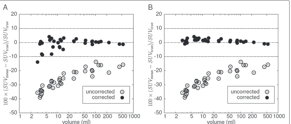
Recovery correction using the true object boundaries

Figure 6 shows the fractional deviation of uncorrected and corrected SUVmean from the known true value for

GBPVC (A) and LBPVC (B) using the true object bound-aries. As expected, the uncorrected data clearly exhibit a reduced mean recovery (down to a recovery coeﬃcient of about 0.6 for the 3 mL lesions). The reduction is size dependent and aﬀects even the largest investigated target structures with volumes of about 500 mL. LBPVC works very good in this case with a deviation of the SUVmean

from the true values of (1.2±1.2) %. Accuracy of GBPVC

Figure 6Deviation of GBPVC-corrected (A) and LBPVC-corrected (B) SUVmeanfrom the true SUVmeanusing the true object boundaries (at

(7)

is comparable to LBPVC for large structures but distinctly inferior for smaller ones with volumes below 20 mL. On average the deviation from the true values is (−1.0±3.8) % for GBPVC.

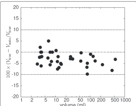
Recovery correction with automatic ROI delineation

The results of the automatic volume delineation are pre-sented in Figure 7 where the fractional deviation of the measured volumes from the true volumes is shown. As can be seen, the derived volumes underestimate slightly the true volumes (by (−3.2 ± 3.1)%). The deviation remains below 10 % in all cases. Figure 8 shows the frac-tional deviation of uncorrected and corrected SUVmean

from its true value for GBPVC (A) and LBPVC (B), respec-tively, when performing automatic volume delineation. The deviation of the LBPVC-corrected SUVmeanfrom the

true SUVmeanalways remains below 10% and equals, on

average,(−0.8±2.5)%. Here, too, GBPVC leads to dis-tinctly larger errors for small target structures, while the deviation for larger objects is comparable to the devia-tion observed with LBPVC. On average the deviadevia-tion is (−2.9±4.5)%.

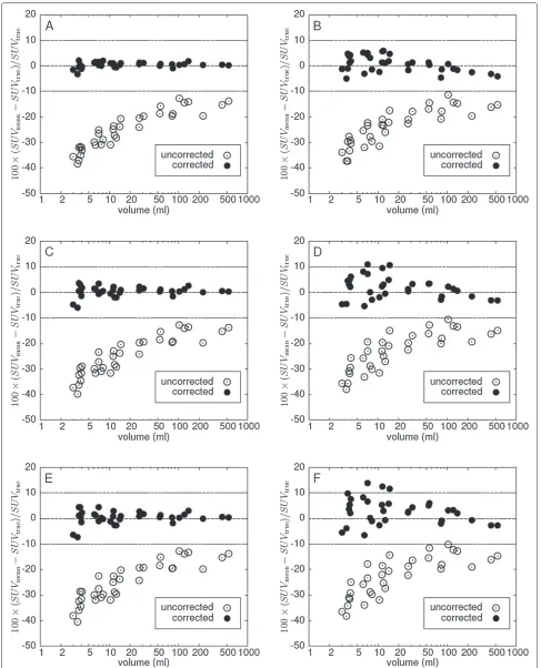
Contrast and noise level dependency

The results of LBPVC for the three investigated additional noise levels are shown in Figure 9. In the left column the true ROI boundaries are used for correction, in the right column automatic ROI delineation is used. Reduced noise (A, B) does not lead to substantially improved results in comparison to Figures 6B and 8B, respectively: on aver-age, the deviation of uncorrected and corrected SUVmean

from its true value is (0.4±1.1) % (A) and (0.7±3.2) % (B), respectively. Elevated noise increases ﬂuctuations of

Figure 7Fractional deviation of the automatically determined object volumes from the true values (at a noise level of FWHM = 5%).Note the logarithmic scale of the abscissa.

the deviations only slightly when using the true object boundaries ((0.4±2.0) % (C) and (0.4±2.6) % (E), respec-tively). On the other hand, LBPVC using the automatic delineation leads to notable noise dependent deviations. However, the deviations always remain below 15% ((1.9

± 4.4) % (D) and (2.9 ± 5.1) % (F) on average, respec-tively). Figure 10 shows the contrast dependence of the diﬀerence between corrected and true SUVmean. The blue

points represent the additional simulated lesions with an artiﬁcially reduced contrast (as described above). The investigated data do not show a systematic dependency on the contrast. Including the additional simulated lesions the deviation of the corrected SUVmean from the true

value is on average (0.8±2.7) %.

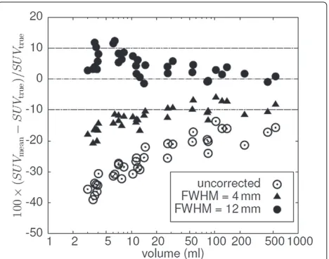
Variation of the assumed spatial resolution

Figure 11 shows results of LBPVC for two diﬀerent val-ues of the assumed FWHM which leads to diﬀerently sized spill-out and background regions: FWHM=4 mm (width of spill-out (background) shell: 1 (2) voxels) and FWHM=12 mm (width of spill-out (background) shell: 3 (5) voxels). Processing the data with an assumed resolution of 4 mm leads to systematic underestimates ((−12±3.6)%) of the necessary PVE correction. Using FWHM=12 mm leads to a slight overestimate ((4.3 ± 3.8)%) of the PVE correction which becomes more dis-tinct for small ROIs.

Discussion

In this paper we present a model-free method for PVE correction of hot focal structures in PET. We have val-idated this method using realistic software phantoms of lesions generated from clinical data. The simulated lesions exhibit properties very similar to those of the underly-ing clinical data sets with respect to relevant parameters (shape/size, contrast, noise, etc.), while having precisely known boundaries and tracer accumulation. The simu-lated data allowed a direct comparison of the PVE cor-rected SUVmeanresulting from automatic ROI delineation

and application of LBPVC with the true SUVmean of

(8)

Figure 8Deviation of GBPVC-corrected (A) and LBPVC-corrected (B) SUVmeanfrom the true SUVmeanusing automatic ROI delineation (at

a noise level of FWHM = 5%).The uncorrected SUVmeanis shown for comparison. Note the logarithmic scale of the abscissa.

shell whose voxels are assumed to be free of any spill-over effects. We have defined these shells in relative units using the estimated spatial resolution FWHM as the rele-vant length unit. Therefore, the assumed resolution does have a certain influence on the accuracy of the correction as demonstrated in Figure 11. If the estimate of FWHM is reduced by a factor of two, the necessary PVE correc-tion is underestimated. This is explained by the fact that the spill-out region becomes too small and not all actually affected voxels are included. In this case, the procedure is therefore not able to collect the complete spill-out signal and, consequently, the correction is too small (especially for small structures).

On the other hand, an increase of the FWHM estimate by a factor of 1.5 results only in a slight overcorrection of the actual partial volume eﬀect and the results are quite similar to those obtained with a realistic FWHM value (deviation from true value(4.3±3.8)%). Only for 4 out of 37 ROIs the deviation was larger than 10 % (but remained below 15 %) if the too large FWHM was adopted. It can thus be stated that the presented method leads to accurate results as long as the actual FWHM is not substantially underestimated. Accurate knowledge of the spatial res-olution is not necessary, however. This is in contrast to e.g. deconvolution techniques [14-19], were the estimated resolution strongly inﬂuences the PVE correction. When in doubt (no accurate knowledge of actual spatial resolu-tion), the best strategy, therefore, is to use a pessimistic (i.e. probably too high) estimate for FWHM, e.g. 8 mm even if actual resolution might be 6 mm.

Our method is similar to the methods discussed in [26,28] with the important diﬀerence that our background approximation is local. This means the contribution of

each voxel in the spill-out region to the PVE correction is computed using the background only in its immediate vicinity (up to a distance of 1.5·FWHM). In this way the method overcomes a limitation of the above mentioned methods which assume a homogeneous background for the whole ROI. In our approach we account for spatial variations of background intensity by determining an indi-vidual background level for each voxel and only assume that the background is homogeneous in the very small background area assigned to the respective voxel (blue area in Figure 2). This is a much weaker and more realistic assumption for most clinical PET studies. The superior-ity of LBPVC over GBPVC can be seen by comparison of Figure 8 (A) and (B). GBPVC (A) leads to reasonable results only for large ROIs (> 20 mL). However, the cor-rected SUVmeanof some of the small ROIs substantially

deviate from the true values and ROI-to-ROI ﬂuctuation is much higher than with LBPVC .

The proposed PVE correction critically depends on a suﬃciently accurate estimate of the true object bound-aries (without such an estimate, speciﬁcation of SUVmean

would not make sense anyway). For this task we used a threshold based automatic ROI delineation (see [29]). With this method we achieved good estimations of the true volume (deviation < 10 %). The observed small deviations of the PVE corrected SUVmean from the true

(9)

Figure 9Diﬀerence between LBPVC-corrected and true SUVmeanat additional noise levels with a FWHM of the Gaussian noise of 3.5% (A,

(10)

Figure 10Contrast dependence of diﬀerence between LBPVC-corrected and true SUVmean.The blue points represent the

subgroup of lesions with artiﬁcially reduced contrast.

to correctly estimate the spill-over contributions from all voxels if the true boundary is known.

This shows, that accuracy of the presented PVE correc-tion is essentially limited only by limitacorrec-tions of the used volume delineation process. Difficulties can, therefore, be expected especially for very small objects with diameter < 2·FWHM [4,5]. In this case correct delineation and, therefore, reliable PVE correction method will certainly fail. A second limitation is the degree of heterogeneity in tracer uptake. Heavily heterogeneous ROIs cannot be delineated correctly with threshold based algorithms [30]. The small but systematic underestimation of the delin-eated ROI volumes shown in Figure 7 can be attributed to this effect. In the present study the heterogeneities of the lesions were moderate (coefficient of intensity vari-ance of voxels within the lesions: 0.13 to 0.22) and the errors in ROI delineation were very small, but it is clear that beyond a certain degree of heterogeneity the method will fail (although such problems can be expected in only a small percentage of the practically relevant cases). Further investigations are necessary to investigate the influence of larger heterogeneities in more detail.

Another factor principally limiting the accuracy of the volume delineation (and of the partial volume correction as well) is a too low contrast of the lesion. However, in our data, covering a contrast range from 2.7 to 13.1, we did not see a clear contrast dependency of the LBPVC correc-tion as demonstrated in Figure 10. Nevertheless, we know from our experience in other investigations that the used delineation algorithm rapidly becomes unstable if the con-trast falls below 2.5. Therefore, the presented correction method will not work reliable for such lesions.

A further factor inﬂuencing the accuracy of LBPVC is the noise level of the image data as demonstrated

in Figure 9. This noise dependency is mainly a con-sequence of decreased accuracy of the volume delin-eation at elevated noise levels. Still, we found that the accuracy remains acceptable even if the noise level is doubled (corresponding to a fourfold decrease of scan time in comparison to our standard acquisition proto-col): in this case only in 3 out of 37 lesions the error exceeds 10% (while remaining below 15%). It is obvi-ous, however, that in the presence of excessive noise (e.g. in single gates from respiration triggered investigations) the presented correction method would not work reli-ably. Since the proposed correction algorithm does not require application of the speciﬁc delineation method used in this investigation, it could also be combined with alternative delineation algorithms with possibly improved performance (notably for heterogeneous structures). The correction method could of course also make use of available morphological information from CT or MRI for very small lesions or lesions with very low contrast, if available.

All investigated lesions with volumes in the range of 3 to 500 mL exhibited substantially reduced mean (as opposed to maximum) signal recovery. That this is the case even for large lesions is explained by the fact that the partial volume eﬀect is a surface eﬀect and the neces-sary PVE correction (regarding SUVmean) remains sizable

even for rather large target structures. The partial volume eﬀect is further increased for irregular/convoluted shapes (compared to approximately spherical objects of the same volume). Irregular shapes are of course not restricted to large structures. In our study sample most lesions with volumes> 10 mL were of distinctly irregular shape (see

Figure 11Diﬀerence between LBPVC-corrected and true SUVmeanusing automatic ROI delineation for diﬀerent values of

(11)

Figure 3). We consider the ability to perform accurate PVE correction for such structures as the most important beneﬁt of the presented algorithm.

For the validation of our method we used simulated target structures which were derived from clinical data. The simulated target structures are much closer to real clinical data than typical (hardware or digital) phantoms. Realistic regional heterogeneities in the target structure or the background are especially difficult to realise (if at all) with the usual phantoms. The same is true regarding the generation/investigation of irregular shapes. More-over, the standard spherical phantom inserts are hollow glass spheres whose cold walls can have a strong influ-ence on the measured partial volume effects [31,32] which are, therefore, not representative for the conditions found in real data. All these problems are avoided by our sim-ulation procedure. For example, although the original tumour uptake heterogeneities are indeed modified by the smoothing applied during the simulation procedure (see above), they remain on a realistic level (see profiles in Figure 4). Despite absence of a true gold standard we believe that the performed validation allows to conclude that the proposed algorithm does provide a means for a quite accurate partial volume correction of real patient data.

The accuracy of the partial volume correction achieved in this study is comparable to the results reported in [18], where an accuracy better than 10% was found for lesions larger than 4 mL. The authors used simulated data and phantom measurements as ground truth and com-pared three diﬀerent correction methods. However, all three investigated methods require a precise knowledge of the true point spread function (PSF) of the tomograph, while in our approach only a rough estimate of the PSF is needed. In [15] accurate correction capability is reported even for very small lesions (diameter 8 mm), but this method, too, requires a precise knowledge of the scan-ner’s PSF. We believe that requiring accurate knowledge of the PSF as a prerequisite is problematic and a potential source of substantial error of the partial volume correc-tion, especially in a clinical context, where data sets might undergo individually diﬀerent postprocessing/smoothing. Our approach, on the other hand is insensitive to variation of the actual PSF within a reasonable range of uncertainty which is an obvious advantage.

Gallivan et al. [8] report on very good results without knowledge of the PSF, but only approximately spheri-cal object with homogeneous tracer uptake were con-sidered, which does not apply to the mostly irregular lesions observed in real patient data. Other authors have proposed to use anatomical information from high res-olution CT or MRI (see e.g. [33-35]). This, however, requires very accurate coregistration of PET and CT/MRI which can be problematic even for modern PET/CT or

PET/MRI systems due to patient motion during mea-surement. Probably more important, this approach rests on the assumption that the morphologically delineated lesion is identical to the hypermetabolic region observed in PET. As is well known, this assumption is by no means always correct. Such a lack of spatial concordance between morphological and functional signal would in turn lead to uncontrollable errors of the PVE correction. In this respect correction procedures relying exclusively on anal-ysis of the PET data alone seem preferable.

We, therefore, believe that the proposed method repre-sents a viable, partly superior, alternative to other methods already discussed in the literature.

Conclusion

The presented approach to partial volume correction using local background determination distinctly improves quantitative accuracy of the correction in comparison to similar, previously described model-free approaches relying on a homogeneous background for the whole lesion. The improvement is especially pronounced for small lesions where the correction becomes numerically large. We conclude that adequate consideration of back-ground heterogeneities on a per-voxel basis is mandatory to achieve reliable partial volume correction.

Competing interests

The authors declare that they have no competing interests.

Authors’ contributions

FH developed and implemented the PVC algorithm, performed part of the data analysis and is the main author of the manuscript. JL and JP performed part of the data analysis. BBB and LO selected the patient studies and performed the lesion delineation in the original patient data. JS and JK provided intellectual input and reviewed the manuscript. JVDH had the initial idea for the voxel based PVC and wrote part of the manuscript. All authors read and approved the ﬁnal manuscript.

Author details

1_{PET Centre, Institute of Radiopharmacy, Helmholtz-Zentrum} Dresden-Rossendorf, Dresden, Germany.2_{Department of Nuclear Medicine, University} Hospital Carl Gustav Carus, Technische Universit¨at Dresden, Dresden, Germany.

Received: 23 January 2012 Accepted: 24 April 2012 Published: 24 April 2012

References

1. Wahl R, Jacene H, Kasamon Y, Lodge M, et al.:From RECIST to PERCIST: Evolving Considerations for PET response criteria in solid tumors.J

Nucl Med2009,50(Suppl 1):122S–150S.

2. Larson S, Erdi Y, Akhurst T, Mazumdar M, Macapinlac H, Finn R, Casilla C, Fazzari M, Srivastava N, Yeung H, et al.:Tumor Treatment Response Based on Visual and Quantitative Changes in Global Tumor Glycolysis Using PET-FDG Imaging: The Visual Response Score and the Change in Total Lesion Glycolysis.Clin Positron Imaging1999, 2(3):159–171.

(12)

4. Hoffman E, Huang S, Phelps M:Quantification in positron emission computed tomography. 1. Effect of object size.J Comp Assist Tomogr 1979,3(3):299–308.

5. Kessler R, Ellis J, Eden M:Analysis of emission tomographic scan data: limitations imposed by resolution and background.J Comp Assist

Tomogr1984,8(3):514–522.

6. Soret M, Bacharach S, Buvat I:Partial-volume eﬀect in PET tumor imaging.J Nucl Med2007,48(6):932.

7. Rousset O, Rahmim A, Alavi A, Zaidi H:Partial volume correction strategies in PET.PET Clin2007,2(2):235–249.

8. Gallivanone F, Stefano A, Grosso E, Canevari C, Gianolli L, Messa C, Gilardi M, Castiglioni I:PVE Correction in PET-CT Whole-Body Oncological Studies From PVE-Aﬀected Images.Nucl Sci, IEEE Trans on2011, 58(3):736.

9. Avril N, Bense S, Ziegler S, Dose J, Weber W, Laubenbacher C, R ömer W, Jänicke F, Schwaiger M:Breast imaging with fluorine-18-FDG PET: quantitative image analysis.J Nucl Med1997,38(8):1186–1191. 10. Präuer H, Weber W, R ömer W, Treumann T, Ziegler S, Schwaiger M:

Controlled prospective study of positron emission tomography using the glucose analogue [18f] ﬂuorodeoxyglucose in the evaluation of pulmonary nodules.Br J Surgery1998,85(11):1506–1511. 11. Geworski L, Knoop B, de Cabrejas, M, Knapp W, Munz D:Recovery

correction for quantitation in emission tomography: a feasibility study.Eur J Nucl Med Mol Imaging2000,27(2):161–169.

12. Aliaga A, Rousseau J, Cadorette J, Croteau É, van Lier J, Lecomte R, B énard F:A small animal positron emission tomography study of the effect of chemotherapy and hormonal therapy on the uptake of 2-deoxy-2-[F-18] fluoro-d-glucose in murine models of breast cancer.Mol Imaging Biol2007,9(3):144–150.

13. Sakaguchi Y, Mizoguchi N, Mitsumoto T, Mitsumoto K, Himuro K, Ohya N, Kaneko K, Baba S, Abe K, Onizuka Y, et al.:A simple table lookup method for PET/CT partial volume correction using a point-spread function in diagnosing lymph node metastasis.Anna Nucl Med2010:1–7. 14. El Naqa, I, Low D, Bradley J, Vicic M, Deasy J:Deblurring of breathing

motion artifacts in thoracic PET images by deconvolution methods.

Med Phys2006,33:3587.

15. Teo B, Seo Y, Bacharach S, Carrasquillo J, Libutti S, Shukla H, Hasegawa B, Hawkins R, Franc B:Partial-volume correction in, PET validation of an iterative postreconstruction method with phantom and patient data.J Nucl Med2007,48(5):802.

16. Kirov A, Piao J, Schmidtlein C:Partial volume eﬀect correction in PET using regularized iterative deconvolution with variance control based on local topology.Phys Med Biol2577,53:2008.

17. Barbee D, Flynn R, Holden J, Nickles R, Jeraj R:A method for partial volume correction of PET-imaged tumor heterogeneity using expectation maximization with a spatially varying point spread function.Phys Med Biol2010,55:221.

18. Hoetjes N, van Velden, F, Hoekstra O, Hoekstra C, Krak N, Lammertsma A, Boellaard R:Partial volume correction strategies for quantitative FDG PET in oncology.Eur J Nucl Med Mol Imaging2010,37(9):1679–1687. 19. van Velden F, Cheebsumon P, Yaqub M, Smit E, Hoekstra O, Lammertsma

A, Boellaard R:Evaluation of a cumulative SUV-volume histogram method for parameterizing heterogeneous intratumoural FDG uptake in non-small cell lung cancer PET studies.Eur J Nucl Med Mol

Imaging2011,38:1636.

20. Brix G, Doll J, Bellemann M, Trojan H, Haberkorn U, Schmidlin P, Ostertag H:Use of scanner characteristics in iterative image reconstruction for high-resolution positron emission tomography studies of small animals.Eur J Nucl Med Mol Imaging1997,24(7):779–786.

21. Reader A, Julyan P, Williams H, Hastings D, Zweit J:EM algorithm system modeling by image-space techniques for PET reconstruction.Nucl

Sci, IEEE Trans on2003,50(5):1392–1397.

22. Alessio A, Kinahan P, Lewellen T:Modeling and incorporation of system response functions in 3-D whole body PET.Med Imaging, IEEE

Trans on2006,25(7):828–837.

23. Vandenberghe S, Karp J:Rebinning and reconstruction techniques for 3D TOF-PET.Nucl Instrum Methods Phys Res A2006,569(2):421–424. 24. Rizzo G, Castiglioni I, Russo G, Tana M, Dell Acqua, F, Gilardi M, Fazio F,

Cerutti S:Using deconvolution to improve PET spatial resolution in OSEM iterative reconstruction.Methods Inf Med2007,46(2):231.

25. Tohme M, Qi J:Iterative image reconstruction for positron emission tomography based on a detector response function estimated from point source measurements.Phys Med Biol2009,54:3709.

26. Hickeson M, Yun M, Matthies A, Zhuang H, Adam L, Lacorte L, Alavi A:Use of a corrected standardized uptake value based on the lesion size on CT permits accurate characterization of lung nodules on FDG-PET.Eur J of Nucl Med Mol Imaging2002,29(12):1639–1647. 27. Verel I, Visser G, Boellaard R, Boerman O, van Eerd, J, Snow G,

Lammertsma A, van Dongen, G:Quantitative 89Zr immuno-PET for in vivo scouting of 90Y-labeled monoclonal antibodies in

xenograft-bearing nude mice.J Nucl Med2003,44(10):1663. 28. Bundschuh R, Essler M, Dinges J, Berchtenbreiter C, Mariss J,

Mart´ınez-M ¨oller A, Delso G, Hohberg M, Nekolla S, Schulz D, et al.: Semiautomatic Algorithm for Lymph Node Analysis Corrected for Partial Volume Eﬀects in Combined Positron Emission

Tomography-computed Tomography.Mol Imaging2010,9(6):319. 29. Hofheinz F, P ¨otzsch C, Oehme L, Beuthien-Baumann B, Steinbach J,

Kotzerke J, van den Hoﬀ J:Automatic volume delineation in oncological PET. Evaluation of a dedicated software tool and comparison with manual delineation in clinical data sets.

Nuklearmedizin Nucl Med2011,51:.

30. Hatt M, Lamare F, Boussion N, Turzo A, Collet C, Salzenstein F, Roux C, Jarritt P, Carson K, Cheze-Le Rest, C, Visvikis D:Fuzzy hidden Markov chains segmentation for volume determination and quantitation in

PET.Phys Med Biol2007,52:3467.

31. Bazanez-Borgert M, Bundschuh R, Herz M, Martinez M, Schwaiger M, Ziegler:Radioactive spheres without inactive wall for lesion simulation in PET.Zeitschrift für medizinische Physik2008,18:37–42. 32. Hofheinz F, Dittrich S, P ötzsch C, van den Hoff J:Effects of cold sphere

walls in PET phantom measurements on the volume reproducing threshold. .Phys Med Biol2010,55(4):1099–113.

33. Rousset O, Ma Y, Evans A, et al.:Correction for partial volume eﬀects in PET: principle and validation.J Nucl Med: Oﬃcial Publ, Soc Nucl Med 1998,39(5):904.

34. Alessio A, Kinahan P:Improved quantitation for PET/CT image reconstruction with system modeling and anatomical priors.Med Phys2006,33:4095.

35. Boussion N, Hatt M, Lamare F, Bizais Y, Turzo A, Cheze-Le Rest C, Visvikis D: A multiresolution image based approach for correction of partial volume eﬀects in emission tomography.Phys Med Biol2006,51:1857.

doi:10.1186/2191-219X-2-16

Cite this article as:Hofheinzet al.:A method for model-free partial volume

correction in oncological PET.EJNMMI Research20122:16.