RESEARCH
A new robust model selection method
in GLM with application to ecological data
D. M. Sakate
*and D. N. Kashid
Abstract
Background: Generalized linear models (GLM) are widely used to model social, medical and ecological data. Choos-ing predictors for buildChoos-ing a good GLM is a widely studied problem. Likelihood based procedures like Akaike Informa-tion criterion and Bayes InformaInforma-tion Criterion are usually used for model selecInforma-tion in GLM. The non-robustness prop-erty of likelihood based procedures in the presence of outliers or deviation from assumed distribution of response is widely studied in the literature.
Results: The deviance based criterion (DBC) is modified to define a robust and consistent model selection criterion called robust deviance based criterion (RDBC). Further, bootstrap version of RDBC is also proposed. A simulation study is performed to compare proposed model selection criterion with the existing one. It indicates that the performance of proposed criteria is compatible with the existing one. A key advantage of the proposed criterion is that it is very simple to compute.
Conclusions: The proposed model selection criterion is applied to arboreal marsupials data and model selection is carried out. The proposed criterion can be applied to data from any discipline mitigating the effect of outliers or deviation from the assumption of distribution of response. It can be implemented in any statistical software. In this article, R software is used for the computations.
Keywords: Arboreal marsupials, Bootstrap, DBC, Robust estimation
© 2016 Sakate and Kashid. This article is distributed under the terms of the Creative Commons Attribution 4.0 International License (http://creativecommons.org/licenses/by/4.0/), which permits unrestricted use, distribution, and reproduction in any medium, provided you give appropriate credit to the original author(s) and the source, provide a link to the Creative Commons license, and indicate if changes were made.
Background
In the last two decades, generalized linear models (GLM) have emerged as a useful tool to develop models from ecological data to explain the nature of ecological phe-nomena. GLM encompass a wide range of nature of response variable like ‘presence-absence’ and ‘count’. It can also be used to estimate the survivorship as can be seen in the conservation literature. GLM builds a dictive model for a response variable based on the pre-dictors. Given a data on response and predictors, the model is fitted using maximum likelihood estimates (MLE) of the unknown regression coefficients. Under certain regularity conditions, the MLE is consistent asymptotic normal estimator of regression coefficients in GLM (McCullagh and Nelder 1989). In the presence of over dispersion, maximum quasi-likelihood estimation
(MQLE) (Wedderburn 1974; McCullagh and Nelder 1989; Heyde 1997) is a popular estimation method. In the process of model building, the researcher may be con-fronted to a pool of predictors of which some might be redundant in nature. If such predictors are included in the model, the response will be predicted with less accu-racy. The fitted GLM may contain some predictors which are redundant in nature and are required to be eliminated from the model based on the observed data.
In the linear regression set up, Murtaugh (2009) evalu-ated the prediction power of various variable selection methods for ecological and environmental data sets. GLM is a wider class of models with linear regression as a particular case when distribution of response is nor-mal. In GLM, there are many methods available in the literature for variable selection. When the likelihood is known, Akaike information criterion (AIC) (Akaike 1974), Bayes information criterion (BIC) (Akaike 1978) and distribution function criterion (DFC) (Sakate and
Open Access
*Correspondence: [email protected]
Kashid 2013) find applications. Sakate and Kashid (2014) proposed a deviance based criterion (DBC) for model selection in GLM which uses MLE of parameters. BIC and DBC are consistent model selection criteria while AIC is not. Sakate and Kashid (2014) empirically established the superiority of DBC over BIC. They also showed that DBC performs better than R¯2 proposed by Hu and Shao (2008).
In practice, the data available for fitting a GLM may be contaminated and the MLE fit of the GLM may not be appropriate. In fact, both MLE and MQLE share the same non robustness property against contamina-tion. Non robustness of MLE in the GLM is extensively studied in the literature (Pregibon 1982; Stefanski et al. 1986; Künsch et al. 1989; Morgenthaler 1992; Ruckstuhl and Welsh 2001). Hence, the use of MLE or MQLE in the presence of contaminated data may give misleading results. The non-robustness of MLE to contamination results in non-robustness of AIC, BIC, DFC and DBC. Hence, using MLE based model selec-tion criterion in presence of contaminated data may be erroneous.
To overcome the problem of contamination in GLM, Cantoni and Ronchetti (2001) introduced robust estima-tion of regression coefficients. Müller and Welsh (2009) proposed a robust consistent model selection criterion by extending the method in Müller and Welsh (2005) to GLM. It is based on a penalized measure of predic-tive ability of GLM that is estimated using m-out-of-n bootstrap method. It is flexible as it can be used with any estimator. Further, Müller and Welsh (2009) empirically established that its performance is best with the robust estimator due to Cantoni and Ronchetti (2001). However, this method is computationally intensive.
In this article, we propose a new robust model selection criterion in GLM. We show that it is a consistent model selection criterion in the sense that as sample size tends to infinity, the model selected coincides with the true model with probability approaching to one. A simula-tion study is presented to compare its performance with its competitors. The proposed model selection criterion along with the other criteria is applied to a data on diver-sity of arboreal marsupials (possums) in montane ash forest (Australia) for model selection.
Results and discussion
An important assumption in the GLM is that the distri-bution of response is a member of exponential family with the general form of the density given by (McCullagh and Nelder 1989)
Pyi;θi,ϕ=e yiθi−b(θi)
a(ϕ) +h(yi,ϕ), i=1, 2,. . .,n
where, θi is the natural location parameter and φ is a scale parameter and yi is the ith observation on the response variable Y.
A GLM is defined via a link function
where, µi=E(Yi)= db(θdθii), XTi is the ith row of n × k matrix X whose first column is of ones and the remain-ing columns contain observations on the predictors X1,X2,. . .,Xk−1 and β=β0,β1,. . .,βk−1T is the vec-tor of regression coefficients.
The log likelihood function is
The maximum likelihood score equations in matrix notations can be written as
where, µ=(µ1,. . .,µn)T. The MLE of regression
param-eter β using iteratively reweighted least squares (IRLS) at convergence is (McCullagh and Nelder 1989)
where, V is an n × n diagonal matrix whose diagonal ele-ments are vi= dµidθia(φ) and ith component of n × 1 vec-tor z is zi=gµˆi+yi− ˆµidgd(µµii).
Robust estimation
The quasi-likelihood estimator is the solution of the sys-tem of estimating equations
where, µ′i= ∂µi
∂β and Q(yi, μi) is the quasi-likelihood function. The solution to Eq. (2) can be viewed as an M-estimator (Huber 1981; Hampel et al. 1986) with score function ψ˜yi,µi
= (yi−µi) V(Yi) µ
′
i. Its influence func-tion (Hampel 1974; Hampel et al. 1986) is proportional to ψ˜ and is unbounded. Therefore, large deviations of the response from its mean or outlying points in the explana-tory variables can have a large influence on the estimator and hence is non-robust (Cantoni and Ronchetti 2001).
Cantoni and Ronchetti (2001) proposed a robust esti-mation procedure based on quasi-likelihood. It is the solution of the estimating equations,
(1) g(µi)=XTi β, i=1, 2,. . .,n
l(β;y)=
n
i=1
yiθi−b(θi)
a(ϕ) +h
yi,ϕ
.
XT(y−µ)=0,
β=X′V−1X−1X′V−1z,
(2) n
i=1 ∂ ∂βQ
yi,µi= n
i=1
yi−µi V(Yi)
µ′i=0,
(3)
n
i=1
ψyi,µi
where, ψyi,µi=vyi,µiw(Xi)µ′i−a(β), a(β)=
1 n
n i=1E
vyi,µiw(Xi)µ′i with expectation taken with respect to the conditional distribution of Y|x , vyi,µi and w(Xi) are weight functions. The constant a(β) ensures Fisher consistency of the estimator. Equation (3) corre-sponds to the minimization of the quantity,
with respect to β where,
with s˜ such that vyi,s˜=0 and ˜t such that Evyj,˜t=0.
Let ri = (√yi−V(µYii)) be the Pearson residual and ψc be the Huber function defined by
where, c is tuning constant. The simple choices for the weight functions v(·,·) and w(·) could be
vyi,µi=ψc(r)√V1(Yi) and w(Xi)=√1−hii, where, hii is the ith diagonal element of the hat matrix. The estimator defined in such a way is called the Mallows’ quasi-likelihood estimator. When w(Xi) = 1, this estima-tor is called as the Huber quasi-likelihood estimaestima-tor. The details on the properties and computational aspect of this estimator are given in Cantoni and Ronchetti (2001).
Robust quasi‑deviance
Cantoni and Ronchetti (2001) introduced the concept of robust quasi-deviance based on the notion of robust quasi-likelihood function to evaluate the adequacy of a model. The robust goodness of fit measure called robust quasi-deviance is defined as
We call the model given in Eq. (1) as full model and denote its sub model as Mα, where α=α0∪αl, α0 = {0} denotes intercept and αl denotes a non empty subset of
1, 2,. . .,k−1. Hence, Mα is an individual model
con-taining the predictors whose suffices are present in the set α. The model Mα, is defined as
(4) QM(y,µ)=
n
i=1 QM
yi,µi
,
(5) QM
yi,µi
=
µi
˜ s
vyi,t
w(Xi)dt
− 1 n
n
j=1
µj
˜ t
Evyj,twXjdt
(6)
ψc(r)=
r, |r|<c, csign(r), |r| ≥c,
(7)
DQM(y,µ)= −2QM(y,µ)= −2 n
i=1 QM
yi,µi
.
(8)
g(µi,α)=XiT,αβα
where, Xi,α denotes the sub-vector of Xi containing com-ponents indexed by α, βα is a pα-vector, and pα denotes cardinality of α. Suppose αN denotes all necessary pre-dictors. Following Shao (1993) and using the notations similar to Hu and Shao (2008), Sakate and Kashid (2013, 2014), we define two exclusive classes of models. If the model Mα contains all the necessary predictors then it is a correct model. Collection of all such correct mod-els is the class of correct modmod-els and is denoted by Mc. Therefore,
Similarly, if the model Mα doesn’t contain at least one necessary predictor then it is a wrong model. Collection of all such wrong models is the class of wrong models and is denoted by Mw. Therefore,
Mw=Mα:at least one necessary predictor is missing,
i.e.Mw= {Mα:αNα} . The model M
α is called the optimal model if it contains only all the necessary predic-tors. It is denoted by MαN. In the following, we discuss robust model selection.
Müller and Welsh (MW) model selection criterion
Müller and Welsh (2009) combined a robust penalized measure of fit to the sample with a robust measure of out of sample predictive ability that is estimated using post-stratified m-out-of-n bootstrap to define a robust model selection criterion A(Mα) in GLM. Let βα be the vector of regression coefficients in the model Mα,g be the link function, ρ be a non negative loss function, δ be a speci-fied function of sample size n, V(Yi)=σ2varXTi,αβα
where, σ2 is a scale parameter and varXT
i,αβα is the vari-ance function and y˜ be a vector of future observations at X that are independent of y. Then the model Mα is selected for which the criterion function (Müller and Welsh 2009)
is small. A common choice of δ(n) is 2 logn (Schwarz 1978; Müller and Welsh 2005). σ2 is usually known. If it is unknown, it is estimated based on the full model by Pear-son Chi square divided by its degrees of freedom. Let β and µ be the estimate of β and μ based on the full model. The in-sample term in the criterion function in Eq. (9) is estimated by σ2
A1(Mα)+1nδ(n)pα
, where Mc=
Mα :all the necessary predictors are present,
i.e.Mc= {Mα :αN ⊆α}
(9) A(Mα)= σ
2
n
E n
i=1
wXi,αρ
yi−g−1
XTi,αβα
σVXT i,αβα
+δ(n)pα
+E
n
i=1
wXi,αρ
˜
yi−g−1XT i,αβα
σVXT i,αβα
y,X
To compute the second term, a proportionally allocated, stratified m-out-of-n bootstrap is implemented. It can be summarized in the following steps (Müller and Welsh 2009).
Step I Compute and order Pearson residuals from the
full model.
Step II Set the number of strata K between 3 and 8
(Cochran 1977, pp. 132–134) depending on
the sample size.
Step III Set stratum boundaries at the
K−1, 2K−1,. . .,(K−1)K−1 quantiles of the
Pearson residuals.
Step IV Allocate observations to the strata in which the Pearson residuals lie.
Step V Sample (number of observations in stratumK)m
n
(rounded if necessary) rows of (y, X)
indepen-dently with replacement from stratum K so
that the total sample size is m.
Step VI Use these data to construct the estimator β∗α,m,
repeat steps V and VI, B independent times
and then estimate the conditional expected
prediction loss by σ2A2(Mα), where
and E∗ denotes expectation with respect to the bootstrap distribution. Combining Eqs. (10) and (11) we get an esti-mate of the criterion function given in Eq. (9) as
Müller and Welsh (2009) suggest using n
4 ≤m≤ n2 for moderate sample size n (50 ≤ n ≤ 200) and if n is large, m can be smaller than n
4.
The robust model selection criterion A(Mα) due to Müller and Welsh (2009) requires computations of the quantities given in Eqs. (10) and (11). Also, a computer intensive proportionally allocated, stratified m-out-of-n bootstrap is required to compute the quantity in Eq. (11). This makes its implementation by a researcher quite
(10) A1(Mα)=
1
n n
�
i=1
w�Xi,α �
ρ
yi−g
−1�XT i,αβ�α
�
�
σV�XTi β��
(11)
A2(Mα)= 1 n
n
�
i=1
w�Xi,α�ρ
yi−g−1�XT
i,α
� �
β∗α,m−E∗ �
�
β∗α,m−β�α
���
�
σV�XT
i �β
�
(12) ˆ
A(Mα)=σ2
A1(Mα)+
1
nδ(n)pα+A2(Mα)
difficult. There is a need of a robust criterion which is easy to implement. We propose a robust version of devi-ance based criterion (DBC) called robust DBC (RDBC).
Proposed robust model selection criterion
The DBC proposed by Sakate and Kashid (2014) is defined as
where, C(n, pα) is a penalty term which measures the complexity of the model.
Instead of deviance, we use robust quasi deviance (Cantoni 2004) as a measure of discrepancy of the fitted GLM. Using the notion behind the DBC, we combine the robust discrepancy measure between a nested model Mα and the full model with the measure of complexity of the model Mα to define a robust model selection criterion in GLM. The robust measure of discrepancy between a nested model Mα and the full model (Cantoni and Ron-chetti 2001) is
where, µα and µ are robust estimators of μα and μ respectively.
We define the robust version of DBC (RDBC) as
RDBC selects the model Mα if RDBC(Mα) is minimum in the class of all possible sub models. In the following, we establish the consistency property of the criterion given in Eq. (14). Note that, ΛQM is always positive and vanishes when Mα is a full model. We require the following condi-tion to establish the consistency property.
Condition 1 For Mα∈Mw and Mα ∗ ∈Mc,
The following theorem ensures that the model selected using RDBC falls in the class of the correct models as n tends to infinity.
Theorem 1 Under the Condition 1, for any correct modelMα∗∈MCand any wrong modelMαwe have,
The proof of the Theorem is deferred to the “Appendix”. The next Theorem establishes the consistency property of DBC(Mα)=
Dy,βα−Dy,β
ϕ −(k−pα)+C(n,pα),
(13)
QM=DQM
y,µα−DQM
y,µ,
(14) RDBC(Mα)=�QM+C(n,pα).
lim n→∞inf
DQMy,µα−DQMy,µα ∗
+C(n,pα)−Cn,pα
∗
>0.
lim n→∞inf Pr
RDBC(Mα) >RDBC
Mα∗
RDBC. Let Mn be the model selected using RDBC when sample size is n.
Condition 2 C(n,pα)=o(n) and C(n,pα)↑ ∞ as n→ ∞.
Theorem 2 Under the Condition 2, with probability approaching to one, as n tends to infinity, RDBC selects the optimal modelMαN
in the class of all correct models
(Mc) i.e.
The proof of the Theorem is deferred to the “Appendix”. RDBC criterion is based on robust estimator which is biased. Therefore, to improve the performance of RDBC, we make use of bias reduction technique like bootstrap to modify RDBC.
Bootstrap RDBC
It is well known fact that the robust estimators of the unknown regression coefficients in the GLM are not unbiased and their bias is non negligible for small to moderate sample sizes. RDBC is based on the robust estimator due to Cantoni and Ronchetti (2001) which is a biased estimator. Therefore, we propose a modified ver-sion of RDBC using proportionally allocated, stratified m-out-of-n bootstrap.
The simulation study in Shao (1996), Wisnowski et al. (2003) and Simpson and Montgomery (1998) indicate that a straightforward implementation of the bootstrap fails in general in the presence of outliers. Müller and Welsh (2005) attributed this partly to non-robust loss function and hence non robust selection criterion and partly to the fact that some of the bootstrap samples may consist almost entirely of outliers. Proportionally allo-cated, stratified m-out-of-n bootstrap was used by Müller and Welsh (2005) for the first time in robust model selec-tion. We propose a modified version of RDBC by replac-ing β by a proportionally allocated, stratified m-out-of-n bootstrap estimate of β. We call this modified version of RDBC as bootstrap RDBC (B-RDBC). It is given by
w h e r e ,�∗QM= 1 B
B
j=1
DQM
y,µ∗
α,m,j
−DQM
y,µ∗
m,j
,
µ∗
α,m,j=g−1
Xα,m,jβ∗α,m,j
,µ∗
m,j=g−1
Xm,jβ∗m,j
and
Xm,j is the jth m-out-of-n bootstrap sample of size m
from the matrix X. To compute the first term in B-RDBC defined in Eq. (15), we use the same algorithm given in section “Results and discussion” with Step VI replaced by Step VI*.
lim
n→∞Pr
Mn=MαN
=1.
(15) B-RDBC(Mα)=�∗QM+C(n,pα),
Step VI* Use these data to construct the estimator
β∗α,m,j, repeat steps V and VI*, B independent
times and then compute ∗QM.
Simulation results
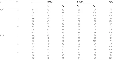
Simulated data is used to compare the performance of the RDBC and B-RDBC with the MW criterion. The simula-tion design used to generate the data is described in detail in the “Methods” section. Table 1 gives the percentage of optimal model selection by RDBC, B-RDBC and MW cri-terion. From the Table 1, it is quite evident that B-RDBC outperforms RDBC for 5 % as well as 10 % contamination for all the sample sizes considered. Use of bootstrapping elevated the optimal model identification ability of RDBC when sample size is small. The performance of B-RDBC with penalty P2 is compatible with MW criterion for small sample sizes. For large sample sizes, the performance of RDBC and B-RDBC with penalty P2 is compatible with MW criterion. As sample size increases, the performance of all the criteria considered in this paper, becomes more or less same. This is because negligible bias is introduced in robust estimates of the regression coefficients when sample size is large. As such, RDBC which is easy to under-stand and implement can be used in place of MW criterion for model selection in GLM when sample size is large.
Real data application
We illustrate the proposed criterion using data on diver-sity of arboreal marsupials (possums) in montane ash for-est (Australia). This data is described by Lindenmayer et al. (1990, 1991) and is a part of the ‘robustbase’ package in R (possumDiv.rda). For details on the study under considera-tion and the data collecconsidera-tion method employed, we refer to Lindenmayer et al. (1990, 1991). The response is the count of different species (diversity) observed on n = 151 sites. Hence, a Poisson regression model is considered. The explanatory variables are shrubs, stumps, stags, bark, acacia, habitat, Eucalyptus and aspect. Cantoni and Ron-chetti (2001) found observation number 59, 110, 133 and 139 as potentially influential data points. In the presence of these influential points in the data, Cantoni and Ronchetti (2001) advocated the use of robust estimator over MLE. We apply the proposed criterion, MW method, AIC and BIC for model selection on arboreal marsupials data. The results are reported in Table 2. B-RDBC and Müller and Welsh method based on Mallows’ quasi-likelihood estima-tor select the same model based on the minimum number of variables. RDBC, AIC and BIC tend to select a model with larger number of variables.
exceedance, ground water contamination, avian popula-tion monitoring, boreal treeline dynamics, aquatic bacte-rial abundance, conservation biology, marine and fresh water fish populations, etc. can be analyzed using GLM. GLM will provide a satisfactory solution to model based inference if only relevant variables are included in the model and there is no deviation from the assumed dis-tribution of response. Identification and safe removal of the redundant predictors from the model in the presence of slight deviation from the assumed distribution of the response can be effectively done by the proposed crite-rion. Our criterion is robust to outliers which are com-mon in any real data. It is also shown to be a consistent model selection criterion. Hence, our criterion is a good
addition to easy implement and consistent model selec-tion toolbox of researchers.
Methods
Simulation design
The empirical comparison of the proposed and existing model selection criteria is done using simulation study. The simulated data was generated according to a Poisson regression model with canonical link (log) and three predictors with intercept i.e. logµi =β0+β1Xi1+β2Xi2+β3Xi3. The predictors were generated from the standard uniform distribution i.e., Xij ~ U(0, 1), j = 1, 2, 3. The observations on the responses Yi’s were generated from Poisson distribution P(μi) and a per-turbed distribution of the form (1−ǫ)P(µi)+ǫP(γ µi), where, ǫ =0.05, 0.10 and γ = 2, 5, 10.
To simulate the data, the regression parameters were set to β0 = 1, β1 = 1, β2 = 2 and β3 = 0. The choice of these parameters is not intentional but only for the pur-pose of illustration. We considered three different sam-ple sizes, n = 64, 128 and 192. To compute B-RDBC and A(Mα), we divided the entire sample into eight equal-sized strata based on the Pearson residuals from the full model. In case of sample size n = 64, we draw 3 obser-vations from each strata with replacement so that the sample size becomes 24. Similarly, for n = 128 and 192, we draw 5 and 7 observations and sample size becomes 40 and 56 respectively. This is in the accordance with the algorithm mentioned in section “Results and discussion”.
Table 1 Percentage of optimal model selection
ǫ γ n RDBC B‑RDBC A(Mα)
P1 P2 P1 P2
0.05 2 64 89 93 98 99 98
128 92 95 99 100 99
192 94 96 100 100 100
5 64 87 93 93 96 99
128 89 93 99 99 100
192 91 93 99 99 99
10 64 86 91 91 96 98
128 91 94 98 99 99
192 92 95 99 99 100
0.10 2 64 88 91 96 98 97
128 90 93 98 99 99
192 92 95 99 100 99
5 64 78 85 78 87 99
128 85 89 94 97 100
192 86 90 96 98 100
10 64 78 83 70 80 98
128 84 88 92 96 99
192 86 91 97 99 100
Table 2 Selected models
Selection criterion Selected variables in the best model
RDBC Stags, bark, acacia, habitat, aspect
B-RDBC Stags, habitat
MW method based on Mallows’
quasi-likelihood estimator Stags, habitat MW method based on bias
cor-rected Mallows’ quasi-likelihood estimator (stratified bootstrap)
Stags, habitat
AIC Stags, bark, acacia, habitat, aspect
In such a way, we obtain B = 50 bootstrap samples for each sample size. To implement RDBC and B-RDBC, we used the penalty functions P1=pαlog(n) and
P2=pαlog(n)+1 for C(n, pα). The Huber score func-tion with tuning constant c = 2 was used to compute the robust estimator due to Cantoni and Ronchetti (2001). It can be easily computed using the robustbase (Rous-seeuw et al. 2014) package in R software. This experiment was repeated 1000 times and the percentage of optimal model selection using these three criteria was obtained.
Appendix
Proof of Theorem 1 Consider,
Therefore using Condition 1 we have, PrRDBC(Mα) >RDBC
Mα∗
=PrDQMy,µα
−DQMy,µα∗
+C(n,pα)−Cn, pα∗>0.
Conclusions
We proposed a robust model selection criterion in GLM called as RDBC. RDBC takes into account goodness of fit as well as complexity of the model. The consistency property of RDBC is also established. Performance evalu-ation and comparison with MW method is done using simulation study. These methods are also applied to the real ecological data. We also defined a bootstrap version of RDBC and called it as B-RDBC. Any suitable pen-alty function can be used without changing the form of RDBC and B-RDBC.
In case of quantitative analysis of environmental and ecological data using GLM, the distribution of response may deviate from the assumed distribution in the model and there might be some redundant predictors pre-sent in the model which are to be identified and safely removed from the model. The proposed criterion can be used effectively to perform model selection in GLM. It is robust to slight deviations from the assumed response distribution and the presence of outliers in the data. Overall, the proposed model selection criterion is robust, consistent and easy to implement model selection crite-rion as compared to its competitors.
Authors’ contributions
DS has defined the proposed method, stated and proved the theorems, performed the simulation study and illustrated model selection for arboreal marsupials data. DK formulated the concept behind the method and contrib-uted in writing, drafting the manuscript and revising it critically for intellectual content. Both authors read and approved the final manuscript.
Acknowledgements
The authors wish to thank the Editor and anonymous referees for their sug-gestions which led to the improvement in the paper.
Competing interests
The authors declare that they have no competing interests. lim
n→∞inf Pr
RDBC(Mα) >RDBCMα∗
= lim
n→∞inf
PrDQMy,µα
−DQMy,µα∗
+C(n,pα)−Cn,pα∗>0
>Prlim n→∞inf
DQMy,µα
−DQMy,µα∗
+C(n,pα)−Cn,pα∗>0=1.
Proof of Theorem 2 In the light of Theorem 1, to prove Theorem 2 it is enough to prove that the value of RDBC for any correct model is larger than that for the optimal model as n tends to infinity. For this consider,
According to Proposition 1 in Cantoni and Ronchetti (2001), DQMy,µαN
−DQMy,µα∗
is distributed as T, where, T is a linear combination of independent Chi square random variables with positive coefficients. Thus, T is a positive valued random variable. Therefore,
Under the Condition 1 and pα∗>pαN, we have,
Cn,pα∗−Cn,pαN
>0 and increases to infinity as n tends to infinity, we have
This indicates that, with probability approaching to one, asymptotically value of RDBC for the optimal model is the smallest in the class of all correct models. Moreover, RDBC selects that model for which its value is minimum among all possible models. Therefore,
□
PrRDBCMα
∗
>RDBCMαN
=PrDQMy,µα ∗
−DQMy,µαN +Cn,pα
∗
−Cn,pαN>0
=PrDQMy,µαN−DQMy,µα ∗
<Cn,pα
∗
−Cn,pαN
PrRDBCMα ∗
>RDBCMα N
=PrT <Cn,pα ∗
−Cn,pα N
lim n→∞
PrRDBCMα ∗
>RDBCMαN=Pr(T <∞)=1
lim
n→∞Pr
Mn=MαN
Received: 23 December 2015 Accepted: 8 February 2016
References
Akaike H (1974) A new look at the statistical model identification. IEEE Trans Autom Control 19:716–723
Akaike H (1978) A Bayesian analysis of the minimum AIC procedure. Ann Inst Stat Math 30:9–14
Cantoni E (2004) Analysis of robust quasi-deviances for generalized linear models. J Stat Softw 10:i04
Cantoni E, Ronchetti E (2001) Robust inference for generalized linear models. J Am Stat Assoc 96:1022–1030
Cochran WG (1977) Sampling techniques, 3rd edn. Wiley, New York Hampel FR (1974) The influence curve and its role in robust estimation. J Am
Stat Assoc 69:383–393
Hampel FR, Ronchetti EM, Rousseeuw PJ, Stahel WA (1986) Robust statistics: the approach based on influence functions. Wiley, New York Heyde CC (1997) Quasi-likelihood and its application. Springer, New York Hu B, Shao J (2008) Generalized linear model selection using R2. J Stat Plan
Inference 138:3705–3712
Huber PJ (1981) Robust statistics. Wiley, New York
Künsch HR, Stefanski LA, Carroll RJ (1989) Conditionally unbiased bounded-influence estimation in general regression models, with applications to generalized linear models. J Am Stat Assoc 84:460–466
Lindenmayer DB, Cunningham RB, Tanton MT, Smith AP, Nix HA (1990) The conservation of arboreal marsupials in the montane ash forests of the Victoria, South-East Australia: I. Factors influencing the occupancy of trees with hollows. Biol Conserv 54:111–131
Lindenmayer DB, Cunningham RB, Tanton MT, Nix HA, Smith AP (1991) The conservation of arboreal marsupials in the montane ash forests of the Central Highlands of Victoria, South-East Australia: III. The habitat require-ments of Leadbeater’s Possum Gymnobelideus leadbeateri and models of the diversity and abundance of arboreal marsupials. Biol Conserv 56:295–315
McCullagh P, Nelder JA (1989) Generalized linear models, 2nd edn. Chapman & Hall, London
Morgenthaler S (1992) Least-absolute-deviations fits for generalized linear models. Biometrika 79:747–754
Müller S, Welsh AH (2005) Outlier robust model selection in linear regression. J Am Stat Assoc 100:1297–1310
Müller S, Welsh AH (2009) Robust model selection in generalized linear model selection. Stat Sin 19:1155–1170
Murtaugh PA (2009) Performance of several variable-selection methods applied to real ecological data. Ecol Lett 12:1061–1068
Pregibon D (1982) Resistant fits for some commonly used logistic models with medical applications. Biometrics 38:485–498
Rousseeuw P, Croux C, Todorov V, Ruckstuhl A, Salibian-Barrera M, Verbeke T, Koller M and Maechler M (2014) Robustbase: basic robust statistics. R package version 0.92-2. http://CRAN.R-project.org/package=robustbase Ruckstuhl AF, Welsh AH (2001) Robust fitting of the binomial model. Ann Stat
29:1117–1136
Sakate DM, Kashid DN (2013) Model selection in GLM based on the distribu-tion funcdistribu-tion criterion. Model Assist Stat Appl 8:321–332
Sakate DM, Kashid DN (2014) A deviance-based criterion for model selection in GLM. Statistics 48:34–48
Schwarz G (1978) Estimating the dimension of a model. Ann Stat 6:461–464 Shao J (1993) Linear model selection by cross-validation. J Am Stat Assoc
88:486–494
Shao J (1996) Bootstrap model selection. J Am Stat Assoc 91:655–665 Simpson JR, Montgomery DC (1998) The development and evaluation of
alternative generalized m-estimation techniques. Commun Stat Simul Comput 27:1031–1049
Stefanski LA, Carroll RJ, Ruppert D (1986) Optimally bounded score functions for generalized linear models with applications to logistic regression. Biometrika 73:413–424
Wedderburn RWM (1974) Quasi-likelihood functions, generalized linear mod-els, and the Gauss–Newton method. Biometrika 61:439–447