Gaussian as Test Functions in Operator Valued Distribution Formulation of QED

http://www.sciencepublishinggroup.com/j/ijamtp doi: 10.11648/j.ijamtp.20180404.12

ISSN: 2575-5919 (Print); ISSN: 2575-5927 (Online)

Gaussian as Test Functions in Operator Valued Distribution

Formulation of QED

Hasimbola Damo Emile Randriamisy

1

, Raoelina Andriambololona

1, *

, Hanitriarivo Rakotoson

1, 2

,

Ravo Tokiniaina Ranaivoson

1

, Roland Raboanary

2

1

Theoretical Physics Department, National Institute for Nuclear Sciences and Technology, Antananarivo, Madagascar

2

Physics and Applications Department, Faculty of Sciences, University of Antananarivo, Antananarivo, Madagascar

Email address:

*_{Corresponding author}

To cite this article:

Hasimbola Damo Emile Randriamisy, Raoelina Andriambololona, Hanitriarivo Rakotoson, Ravo Tokiniaina Ranaivoson, Roland Raboanary. Gaussian as Test Functions in Operator Valued Distribution Formulation of QED. International Journal of Applied Mathematics and Theoretical Physics. Vol. 4, No. 4, 2018, pp. 98-104. doi: 10.11648/j.ijamtp.20180404.12

Received: November 9, 2018; Accepted: December 3, 2018; Published: January 25, 2019

Abstract:

As shown by Epstein and Glaser, the operator valued distribution (OPVD) formalism permits to obtain a non-standard regularization scheme which leads to a divergences-free quantum field theory. The present formulation gives a tool to calculate finite scattering matrix without adding counter-terms. After a short recall about the OPVD formalism in 3+1-dimensions, Gaussian functions and Harmonic Hermite-Gaussian functions are used as test functions. The field resulting from this approach obeys the Klein-Gordon equation. The vacuum fluctuation calculation then gives a result regularized by the Gaussian factor. The example of scalar quantum electrodynamics theory shows that Gaussian functions may be used as test functions in this approach. The result shows that the scale of the theory is described by a factor arising from Heisenberg uncertainties. The Feynman propagators and a study on loop convergence with the example of the tadpole diagram are given. The formulation is extended to Quantum Electrodynamics. Triangle diagrams anomaly are calculated efficiently. In the same approach, using Lagrange formulae to regularize the singular distribution involved in the scattering amplitude gives a good way to avoid infinities. After applying Lagrange formulae, the test function could be reduced to unity since the amplitude is regular. Ward-Takahashi identity is calculated with this method too and this shows that the symmetries of the theory are unbroken.

Keywords:

Quantum Electrodynamics, Triangle Anomaly, Ward-Takahashi Identity, Partition of Unity, Operator Valued Distribution, Gaussian Functions, Tadpole Diagram

1. Introduction

Divergences appear when calculating S-matrix in Quantum Theory [1-3]. Many approaches have been considered to deal with this problem.

The standard renormalization techniques based on the dimensional regularization and Cut-Off method has been used [1, 2, 4]. Operator Valued Distribution approach (OPVD) developed by Epstein and Glaser [5] based on the mathematical theory of distribution is considered in this

paper.

In this work, the quadri-momentum is denoted by ̅

0,1,2,3 where is a basis in the Minkowski space and the tri-momentum by 1,2,3 in which is the 3-dimensional Euclidian basis. The corresponding scalar products are . ̅ and .

.

In the Minkowski space with signature 1, 3 , the field is defined by

in which

is a test function

Φ is an OPVD [5-9]: it is an operator on a Fock space and a distribution acting on the set of test functions.

̅is the translation operator defined by the relations

! ̅ "# "# + ̅

〈 ̅Φ, 〉 〈Φ, % ̅ 〉 The explicit expression of the field is [7]

, & '_+√-./()*)_√-10 23 % *̅. ̅+ 45 *̅. ̅6 7 8, (2)

in which

3 and 45 are respectively particle annihilation and antiparticle creation operators satisfying the commutation relations

923 , 4

5 _{: 6 23 , 4 : 6 0}

23 , 35 _{: 6 ;}< _{− :}

24 , 45 _{: 6 ;}< _{− :}

(3)

8 > ? -+ @- is the energy of a free particle, @ being its mass.

Ais the Fourier transform of the test function

7 ̅ _+√-./0 B' "# % *̅.C#DE"# (4)

The Klein-Gordon equation

F F − @- _{̅ 0 (5)}

for 0, … ,3 is satisfied. The cases in which the test functions are Gaussian functions namely Harmonic Hermite-Gaussian functions introduced in the references [10-12] are studied. Denoting the latter _H and their Fourier transforms 7_H their expressions are

I H ̅ JH ̅ %ℬLM L%NL M%NM% OL L

7H ̅ ℛH ̅ %QLM+*L%OL/ *M%OM R NL*L%OL

(6)

in which J_H ̅ and ℛ_H ̅ are polynomials of degree S respectively withvariables and variables ,

0,1,2,3 . T and U are respectively the mean values of the variables and

I'_{'| 7}| H ̅ |-DE ̅ 1 ' | H ̅ |-DE ̅ T

H ̅ |-DE ̅ 1 ' | 7H ̅ |-DE ̅ U (7)

Q W _{and ℬ W are the components of second order tensors} representing the coordinate and momentum dispersion-codispersion operators corresponding to the ground state (n=0) [11-13].

X

' − T W_{− T}W _|

> |-DE ̅ Q W

' − U W− UW | 7> |-DE ̅ ℬ W

Q Y_ℬ

YW 0_E;W

(8)

The polynomials J_H ̅ and ℛ_H ̅ in the relation (6) can be expressed in terms of Hermite polynomials [11].

For the case Q W ℬ _W 0 for ≠ [, the uncorrelated Harmonic Hermite Gaussian functions are

\ ] ^ ]

_JH ̅ ∏

a_bLcLdeL ?fQLL g-bL_HL_{! √-.})ij_√QLL <

k>

ℛH ̅ ∏

a_bLlLdmL_√fℬLL

g-bL_HL_{! √-.})ij_?ℬLL <

k>

(9)

in which n_HL is the Hermite polynomials of degree S . For the ground state, S 0 0,1,2,3, the relations 6 give

\ ] ^ ]

_ > ̅ p

dℬLM+cLdeL/+cMdeM/dqmLcL

g+√-./)ij∏)_Lrs√QLL

7> ̅ pdQLM+lLdmL/ lMdmM iqeL lLdmL g+√-./)ij∏)Lrs?ℬLL

(10)

2. Gaussian Functions as Test Functions

In this section, the case in which the test function is the Gaussian function 7_> ̅ is considered. For sake of simplicity one chooses T 0. This approach is suggested by the fact that Gaussian functions correspond to the normal probability distribution and appear in the modeling of many phenomena.

2.1. Calculation of Vacuum Fluctuation

The vacuum fluctuation is given by

t ̅, "# u0v ̅ 5 _{"# v0w (11)}

|0〉 being the vacuum state and

5 _{"# '} ()* +√-./)

0

√-1235 *̅.C#+ 4 % *̅.C#6 7> 8, (12)

then

t ̅, "# '_+√-./()*) ( )_xy +√-./)

0

-1u0v3 35 : v0w % *̅. ̅%C# × 7> 8, 7> 8′, : (13)

The integration of 14 over : gives

t ̅, "# '_{-1 -.}()*) % *̅. ̅%C# 2 7> 8, 6- (15)

This result (15) differs from the classical one by the regularizing factor 2 7_> 8, 6-.

Using the expression of 7_> in the relation (10) and taking the case _> 8 one has explicitly

t ̅, "# '_{-1 -.}()*) % *. ̅%C# p

dfQLM lLdmL lMdmM

+√-./)∏)Lrs?ℬLL (16)

2.2. Calculation of Feynman Propagator

The Feynman propagator in the configuration space is

Δ~ ̅ − "# − u0v• ̅ 5 "# v0w (17) in which • is the chronological product [1].

• ̅ 5 _{"# I} ̅ 5 "# >€ ">

5 _{"# ̅ "}>_€ > (18)

Then

u0v• ̅ 5 _{"# v0w • & u0v ̅} 5 _{"# v0w + • −& u0v} 5 _{"# ̅ v0w (19)}

in which & >− "> in natural units (‚ 1) and • is the Heaviside function.

The expressions (1.2) and (2.2) of fields give

u0v• ̅ 5 _{"# v0w '} (B*̅ -.B 2ƒ7s* 6

f_pdql. cd„

2 *s f_%+1l/f_{R …6} (20)

' (_-.B*̅B 2ƒ7s* 6 f

2 *s f_%*f_%†f_{R …6} % *̅. ̅%C# (21)

The Feynman propagator in the configuration space is

Δ~ ̅ − "# ' ( B_*̅ -.B p

dql. cd„ 2*̅f_%†f_{R …6}×p

dfQLM lLdmL lMdmM +√-./B∏)Lrs?ℬLL (22)

The Feynman propagator in momentum space is

∆ˆ~ ̅ _2*̅f_%†0f_{R …6}p

dfQLM lLdmL lMdmM

+√-./B∏)Lrs?ℬLL (23)

3. Harmonic Hermite-Gaussian

Functions as Test Functions

The Harmonic Hermite-Gaussian functions defined in the relation (6) are taken as test functions. The vacuum fluctuation and the Feynman propagators (with T

0 and > 8 are in this case

u0v ̅ 5 _{"# v0w '} ()*

-1 -.) % *̅. ̅%C# × ℛH 8, p

dfQLM+lLdmL/ lMdmM

+√-./B∏)Lrs_+?ℬLL/ (24)

Δ~ ̅ − "# ' ( B_*̅

-.B_2*̅f_%†0f_{R …6} % *̅. ̅%C# × ℛH ̅ p

dfQLM+lLdmL/ lMdmM

+√-./B∏)Lrs+?ℬLL/ (25)

∆ˆ~ ̅ _2*̅f_%†0f_{R …6}ℛH ̅ p

dfQLM+lLdmL/ lMdmM

+√-./B∏)Lrs_+?ℬLL/ (26)

The difference between the expressions (11), (13) and (24), (25), (26) is the presence of the polynomialsℛ_H ̅ which is reduced to a product of Hermite polynomials in the case of uncorrelated variables.

4. Application to One Loop Scalar

Quantum Electrodynamics Diagram

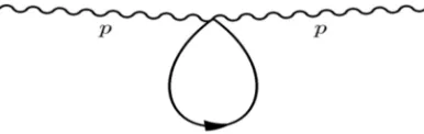
One loop scalar tadpole diagram contributes to the two points correlation function. The associated amplitude is calculated since it is simple and the regularization factor appears.

4.1. Divergence in the Framework of Standard Formulation

The above results may be applied for the calculation of more complicated entities considered in the scalar field theory. For instance for the calculation corresponding to the tadpole diagram which appear in the calculation of photon propagator in conventional scalar QED [1]

In the old formulation, the amplitude of this tadpole diagram is given by

‰W 2 - W' ( B_Š#

-.B_Š#f_%†f_{R ‹} (27)

Introducing quadridimensional spherical coordinate Œ_•, t, •, Ž , the relation (27) becomes

‰W p

f_ƒLM

•.B ' ' ' ' Š•

) Š•fR†f -. > . > . > R‘

> ’ St - ’ S• DŒ•D•DtDŽ p

f_ƒLM E.f “Š•

f

- +

†f - ln –

Š•f †f + 1—˜_>

R‘

(28)

where

Œ•- Œ>-+ Œy

-The expression (28) shows quadratic and logarithmic divergences. In the standard formulation, one deals with this divergence using regularization and renormalization techniques [1- 2].

4.2. Calculation in the Framework of OPVD Formulation Using Gaussian Functions

Let us now use the Gaussian functions defined in the relation 1.6 . The Feynman propagator in momentum space is given by the relation (23). The analog of the integral (27) is then

‰W 2 - W'( B_Š•

-.B_Š•f0_R†f 2 7>+Œ•-/6- (29)

As the main interest is the study of convergence, one considers the case

X

Q W _{0 ≠ [}

Q Q _Eℬ0

™ 0

(30)

The integral (29) becomes

‰ W 2 - W'( B_Š•

-.B_Š•f0_R†f % š•f

fℬ (31)

then

‰ W 4›- - W' Š• )_pdš•_fℬf Š•fR†f R‘

> DΥ (32)

Performing the variable change œ Š•

√-ℬ, leads to

‰W p

f_ƒLMℬ

-.f ' •

)_pdžf •f_R Ÿ

√ℬf R‘

> Dœ (33)

Following the interpretation in the references [11-13], the parameter √ℬ is the common value of the uncertainty (statistical standard deviation) on the values of the energy Œ_> and the components Œ ¡ 1,2,3 of the spatial momentum of the particle corresponding to the tadpole. In the very large

energy approximation, †

√ℬ -→ 0, the integral (33) becomes

‰W p

f_ℬ

-.f W' œ_>R‘ %•f Dœ p f

E.f ℬ W (34)

As expected, the result is obtained is finite. This result relates explicitly the existence of loop in the photon propagator of scalar QED to the Heisenberg uncertainty relation. This relation is obvious since the Heisenberg principle is already integrated in the representation of quantum phase space formalism.

5. Triangle Axial Anomaly in QED

Let us use Gaussian test function to calculate diagram in QED which involved current conservation. Axial anomaly can be understood by calculating the two triangles graphs

Figure 2.One loop triangle diagrams.

The amplitude of the two graphs contributing to the triangle anomaly can be written as [2]

•Š,£, 0, - ¤Š,£,0 0, - + ¤£,Š,- 0, - (35)

¤Š,£,0 0, - represents the amplitude of the first diagram in Figure 2 and ¤_£,Š,- ₀, _- represents the amplitude of the second diagram in Figure 2.

The conservation of the axial currents at the vertices will be shown [2]

0+ - •Š,£, 0 (36)

Using Feynman rules and after some algebra calculation the amplitude is equal to

0+ - +¤Š,£,0 + ¤Š,£,- / 4 ²¦§£¨Š© D E_Œ#

2› EŒ ¨

9Δ 7 7 –

Š#f -ℬ— “ 7 –

Š#%*̅f f -ℬ — − 7 –

Š#R*̅f -ℬ —˜

Δ 7′ 7 –_-ℬŠ#f— “ 7 –Š#R*̅j f -ℬ — − 7 –

Š#%*̅j f

-ℬ —˜

(37)

The result 37 shows that relation 36 is satisfied in the limit where ̅₀-, ̅_--≪ 2ℬ. In this limit too, 7 depends only on the Œ- variable everywhere

9Δ 7 7 –

Š#f -ℬ— “ 7 –

Š#f -ℬ— − 7 –

Š#f -ℬ—˜ 0

Δ 7¬ _{7 –}Š#f -ℬ— “ 7 –

Š#f -ℬ— − 7 –

Š#f -ℬ—˜ 0

(38)

The conservation of the axial current is then verified by our canonical regularized quantum field.

It may be shown that the conservation of the axial current is kept in general case (see section 6).

In the following, another Gaussian type function is used and the introduction of a partition of unity [5] generalizes the results.

6. Field as OPVD with Gaussian Test

Function

The amplitude in the OPVD formalism is

- ' DT • T_>‘ T (39)

where T is the Gaussian test function. The calculation will be done in one dimension for the sake of simplicity. Four-dimensional extension can be achieved using integration by part.

6.1. Gaussian Test Function as Partition of Unity

One reduces the test function to a partition of unity following the procedure in [5-7] by the convolution of the Gaussian function of the form

!® % f ‖ ‖ < 1

0 ±’ ²ℎ (40)

where ® is a normalization factor. The test function as partition of unity will be denoted and it can be tend to 1 over the whole domain in a given limit.

6.2. Construction of the Distribution Extension in the UV Limit

In this section, Lagrange formula is used for the case of large momentum. In quantum field theory, the amplitude associated to the Feynman diagrams could be defined as

- ' DT •´‘ µ _{T T}

> (41)

where •´µ T is the extension of the distribution• T in the UV limit. This amplitude Q is regularized by the Gaussian test function.•´µ T is useful in higher order calculation since it is regular.

6.3. Extension of the Test Function

In order to avoid the pole in the amplitude, the test function is modified using the Taylor remainder [5]. In the UV limit, the test function is equal to its Taylor remainder

µ _{T −}N

Š!'

(¶ ¶ ·f¸¹ ‖N‖

0 1 − & ŠFNŠR0+TŠ µ T& / (42)

Here, the upper born, º-»_¼ ‖T‖ , is given by the arbitrary choice of a running support. Following the procedure described in [5], one changes µ T for this value and get

- − © DT • T _{Œ! ©}T · D&_&

f_¸¹‖N‖

0 1 − &

Š ‘

> FN

ŠR0_+TŠ µ _{T& /}

6.4. Extension of the Distribution ½ ¾

Integrating by parts 6.5 and performing the limit µ _{T& → 1, which is now possible since the distribution is} regularized, the definition of the extension of the distribution in the UV domain [4, 5, 6] is now given by

•´µ _T %Nš

Š! FNŠR0+T• T / ' (¶

¶ ·f

0 1 − & Š (43)

This Lagrange formula gives a divergence-free contribution.

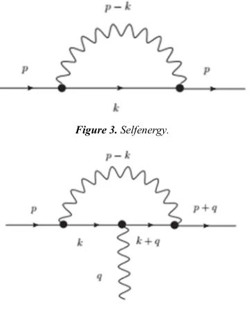
7. Ward-Takahashi Identity

In order to keep the gauge symmetry of the theory, one calculates the Ward-Takahashi identity in one loop order. This identity is given by [2]

;À −_{Á Â*}Á Ã Ä Å

Â*k† (44)

Figure 3. Selfenergy.

Figure 4. One loop Vertex.

One uses the Lagrange formula described above to calculate the two diagrams amplitude.

7.1. One loop Self-energy Diagram

The corresponding amplitude is obtained by using

Feynman rules

Ã Ä © D_2›EŒ#_E Ä Œ + @_{Œ#-− @-} ļ −

+ ̅ − Œ#/-− ²Ä¼ +Œ#-/ –+ ̅ − Œ#/

-_—

in which

1 Œ# is the quadri-momentum

2) is a factor emerging from the field formulation as Operator Valued Distribution. A photon mass is introduced to avoid IR-divergence [2].

3) Ä_¼ are the Gamma matrices of Dirac

Introducing the Feynman parameterization, the integral becomes

à Ä

© D © D_2›EŒ#_E 2 Ä ̅ − 4@ +Œ#-_{− Æ}- _{, ̅² /}

--_Ç ̅. ̅

Λ-É -ÊŒ#

-Λ-Ë 0

>

where

Æ- _{, ̅}- _{1 − ̅}-_{+ @}-_{+ 1 −}

-and Λ is an arbitrary scale which is related to the dispersion parameter. In order to use the Taylor formula one makes the variable change T Œ-/Λ

-Then

Ã Ä _0Í.²p² ' D Î2 Ä_>0 − 4@Ï' FN N f NR0fDT R‘

> ±S –Ðf·²_,*̅f— -–TÐ f_Ñ,*̅f

Ò² — (45)

The integral can be split into the following integrals

\ ] ^ ]

_ ¤0 1 ' DT _>‘ _NR00 -–TÐ f _,*̅f

Òf —

¤- −3 ' DT _>‘ _NR00 f -–TÐ f _,*̅f

Òf —

¤< 2 ' DT >‘ _NR00 ) -–TÐ f _,*̅f

Òf —

(46)

The application of the Lagrange formula gives

Ã Ä −_E.¼ ' D Î2 Ä_>0 − 4@ϱS _{0% *̅}f_{R †}·fÒff_{R 0%} f (47)

The self-energy diagram contribution thus obtained is the same as in the dimensional regularization procedure. The Ward-Takahashi identity is related to the derivative of the self-energy.

ÁÓ Â*

Á Â* Å_Â*k† −

¼

E.“±S –º- Ô f

†f— − 2±S – f

†f—˜ + Õ –† f Ô²,

f Ô²— (48)

This result is equivalent to those obtained by conventional calculation up to a constant term which could be introduced in the logarithmic part by some basics properties.

7.2. Vertex Diagram

The last diagram which contributes to the Ward identity in QED at one loop order is the vertex diagram. It involves the coupling between fermion and photon, with a radiative

correction [1-2].

The distribution part of the amplitude is equal to

;Γ ' (_-.BŠ#B _Š#%*̅0f_R fÄW +Â L_ŠLR†/ Š#Rx# ²%†fÄ +Â

L_ŠLRÂL_xLR†/

Š#f_%†f ÄW (49)

The matrix identities

I_ļ_± ÄWÄ ÄW −2Ä

¼Ä Ä×±× 2± ±WÄW− Ä ±Y±Y (50)

and the Feynman parametrization lead to the vertex contribution

;Γ _-.¼' DØ 1 − Ø>0 ' ( B_Ù̅ -.B

“%j_fÂL_Ù̅f_{RO Ñ †}f_ÂL_˜ 2Ù̅f_%Ðf6) R‘

%‘ Œ + Ø ̅- (51)

-After a variable change and introducing a dimensionless variable X, the expression (51) becomes

;Γ _-.¼ ' DØ 1 − Ø_>0 ' DT >‘ N N%0_2NR06) -–TÐ f_Ñ,*̅f

Ôf — (52)

The method analog to the self-energy calculation may be applied and leads to the expression

;À _E.¼ “±S –·_†fÔff— − 2 ±S – f

†f—˜ + Õ –† f Ôf,

f

Ôf— (53)

This result is equivalent to those obtained in others regularizations procedure. In our case the Ward-Takahashi identity was verified since

;À −ÁÓ Â*_{Á Â*} Å

Â*k† ¼

E.“±S –º- Ô f

†f— − 2±S – f

†f—˜ + Õ –† f Ô²,

f

Ô²— (54)

This equation proves that introducing Gaussian as test function reduced to partition of unity provide, at one loop order, self-energy and vertex satisfying the Ward-Takahashi identity.

8. Conclusion

It is shown that Gaussian functions may be used as test function in OPVD formulation of a Quantum Field Theory to deal with divergence. QFT is then defined, not in point space-time but smeared in an area described by the Gaussian test function. The quantum scalar fields obey Klein-Gordon equations due to the properties of test functions. One obtains expressions of the vacuum fluctuation and Feynman propagators which contain Gaussian regularization factor. The Loop calculation is performed in the case of one loop tadpole diagram and divergence-free result was obtained.

The Gaussian functions have some mathematical and physical properties which may make this approach interesting. The Heisenberg uncertainty principle is incorporated and it is represented by the factor ℬ. The case in which the mass m ≪ √ℬ is considered and yields finite result. The amplitude is related to the value ℬ of the dispersion (statistical variance) of the energy and components of spatial momentum. The standard QFT corresponds to a large value of ℬ. The main advantage of this formulation is that it needs no counter-parts to treat divergences in the higher order in perturbation theory. The dimension of space-time is not modified like in the dimensional regularization.

The test function is also reduced in partition of unity. After applying the Taylor formula in the singular distribution, one obtains finite amplitude. Gauge and Poincaré invariance is verified at one loop level and it is the case for the Ward-Takahashi identity too.

References

[1] Matthew Schwartz “Introduction to Quantum electrodynamics”, Harvard University, Fall 2008.

[2] Lewis H. Ryder “Quantum electrodynamics”, Cambridge University, 1985.

[3] Mikhaïl Shaposhnikov, Champs Quantiques Relativistes, Sven Bachmann, 2005.

[4] H. Kleinert and V. Schulte-Frohlinde, Critical Properties of scalar theories November 22, 2016.

[5] Jean-François Mathiot, Toward finite field theory: the Taylor– Lagrange regularization scheme, 2012.

[6] Bruno Mutet, Pierre Grangé and Ernst Werner, Taylor Lagrange Renormalization Scheme: electron and gauge-boson self-energies, (PoS) Proceeding of Science (2010).

[7] Pierre Grange, Ernst Werner. Quantum Fields as Operator Valued Distributions and Causality. 20 pages, 2 figures - Contrat-IN2P3-CNRS.<hal-00118075v2>, 2007.

[8] Laurent Schwartz, Théorie des distributions, Hermann, Paris 1966.

[9] Günther Hormann& Roland Steinbauer, Theory of distributions, Fakultat fur Mathematik, Universitat Wien Summer Term 2009.

[10] Ravo Tokiniaina Ranaivoson, Raoelina Andriambololona, Rakotoson Hanitriarivo. Time-Frequency analysis and harmonic Gaussian functions. Pure and Applied Mathematics Journal. Vol. 2, No. 2, 2013, pp. 71-78. doi: 10.11648/j.pamj.20130202.14, 2013.

[11] Ravo Tokiniaina Ranaivoson: Raoelina Andriambololona, Rakotoson Hanitriarivo, Roland Raboanary: Study on a Phase Space Representation of Quantum Theory, arXiv: 1304.1034 [quant-ph], International Journal of Latest Research in Science and Technology, ISSN (Online): 2278-5299, Volume 2, Issue 2: pp. 26-35, March-April 2013.

[12] Ravo Tokiniaina Ranaivoson, Raoelina Andriambololona, Hanitriarivo Rakotoson, Properties of Phase Space Wavefunctions and Eigenvalue Equation of Momentum Dispersion Operator, arXiv: 1711.07308, International Journal of Applied Mathematics and Theoretical Physics. Vol. 4, No. 1, 2018, pp. 8-14, 2018.